"Sorting" <=> "Rubyists"

This talk is not for people who studied computer science. If you know what Big O Notation is, you can leave now. I have nothing to give to you.

.. This is for you folks who call #sort and have no idea what demon is moving your strings around in an array, but you get that array back sorted and that’s pretty cool.

.. This is for you folks who call #sort and have no idea what demon is moving your strings around in an array, but you get that array back sorted and that’s pretty cool.

Algorithms To understand what Ruby or Postgresql do when you sort an array, let’s talk about algorithms.

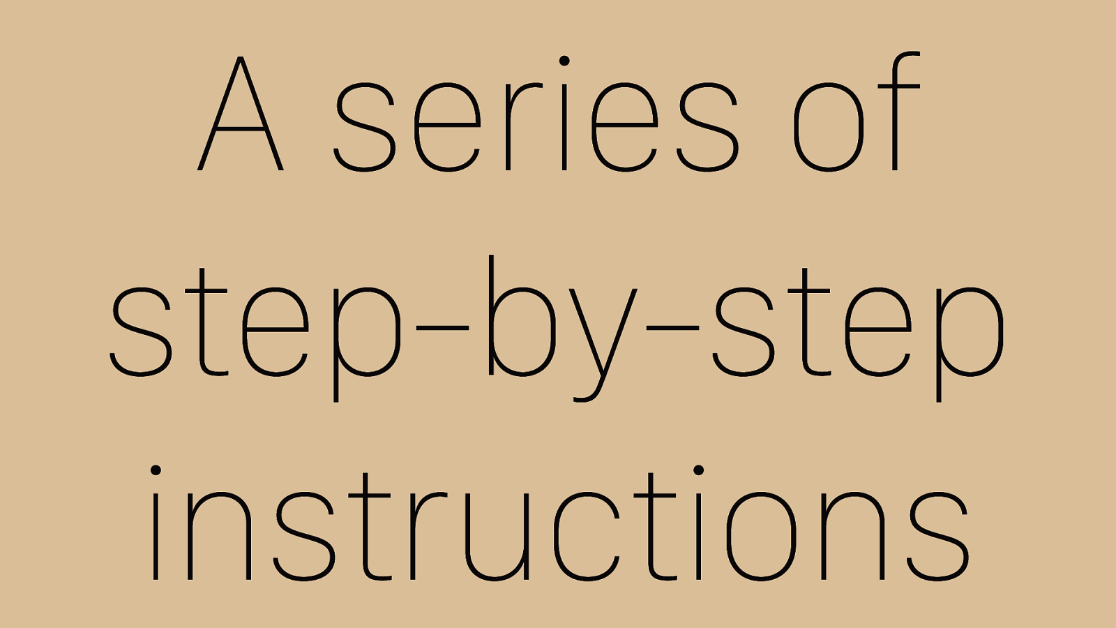
A series of step-by-step instructions It’s a scary word, but all it means is a series of step-by-step instructions to complete a task.

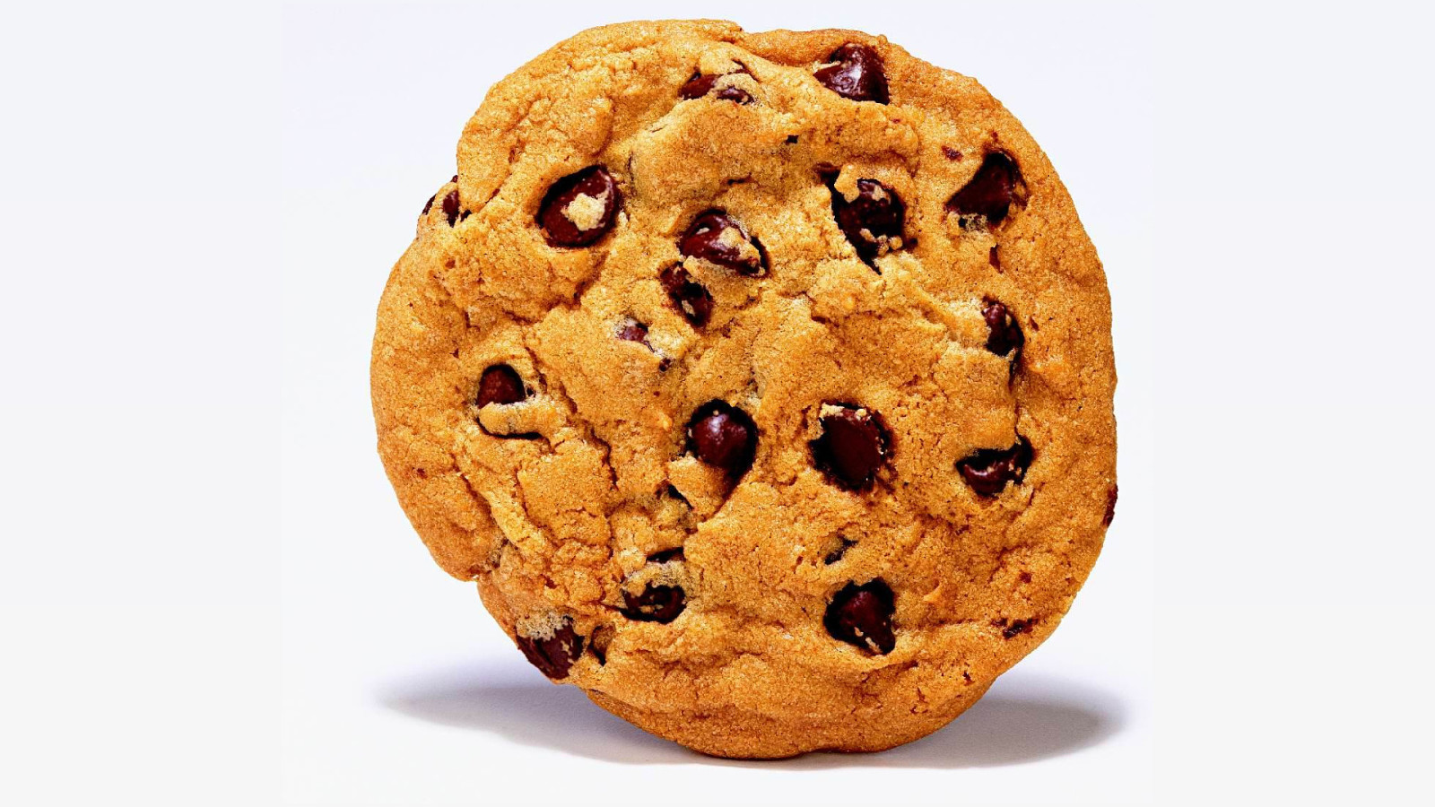
t A recipe for chocolate chip cookies is an algorithm. I didn't have to understand the chemistry and gastronomy of the instructions. When I realized this was a good example, I just found a recipe for chocolate chip cookies and made a batch immediately before I kept going. I followed directions and ended up with delicious cookies that I ate all of.

:14

Big O Before we get too far, I want to talk about Big O. Big O can be a scary concept when you see it written out. I usually assume it’s something for math people and I make websites, so that’s probably not me. But when it comes down to it, Big O isn’t really that scary.

Big O is how we answer “How fast is an algorithm” and use that answer to compare algorithms to each other.

It is based on the assumption that basic operations involved in an algorithm will take the same amount of time between algorithms that perform the same task.

This allows us to compare using # of operations as a function of the inputs instead of time to complete.

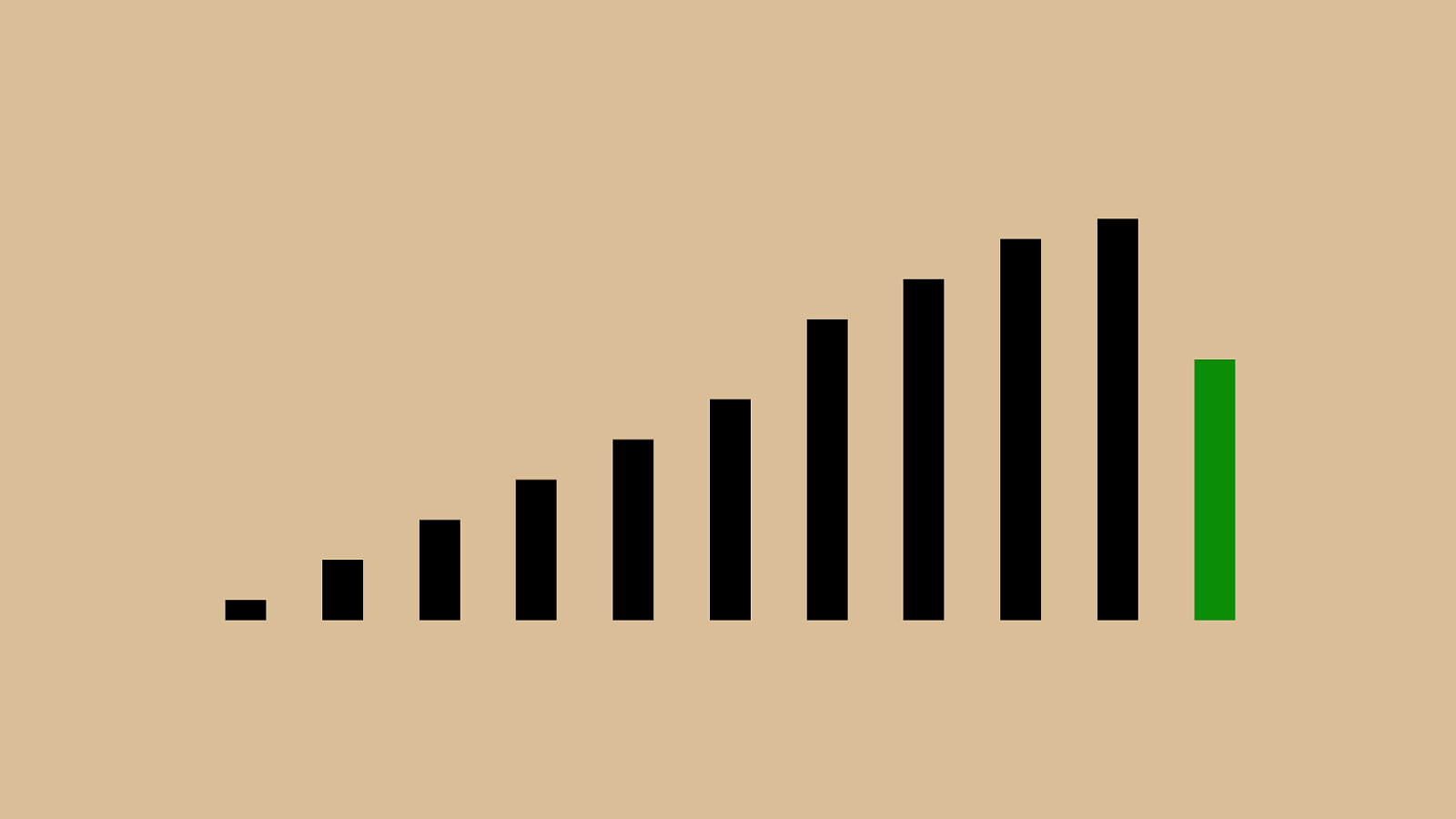
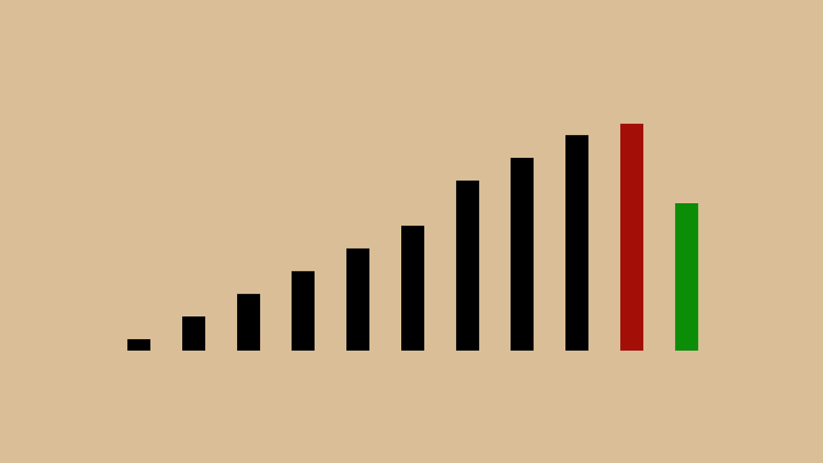
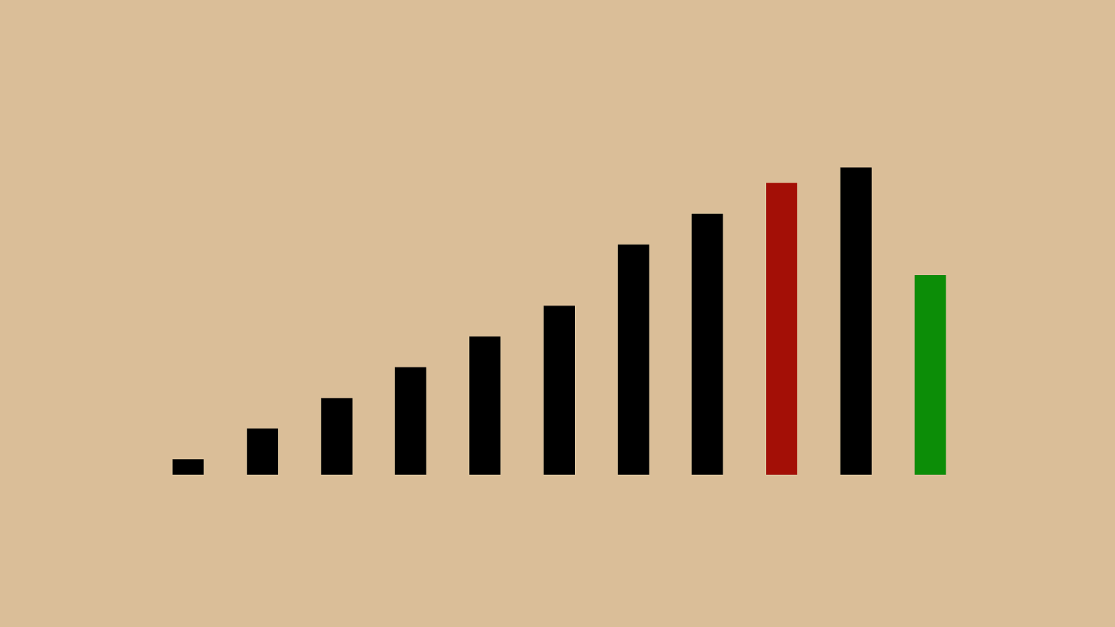
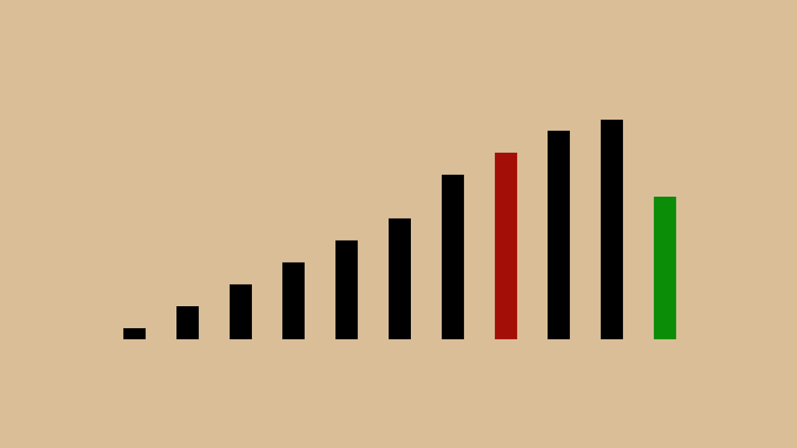
Let’s look at a couple of algorithms for cutting out squares from this paper.

When I previously gave this talk, I got a lot of feedback that the audience couldn’t see what I was cutting out since I used pretty small pieces of paper. So of course, I bought big-ass scissors, a giant pad of post it notes, and an easel.

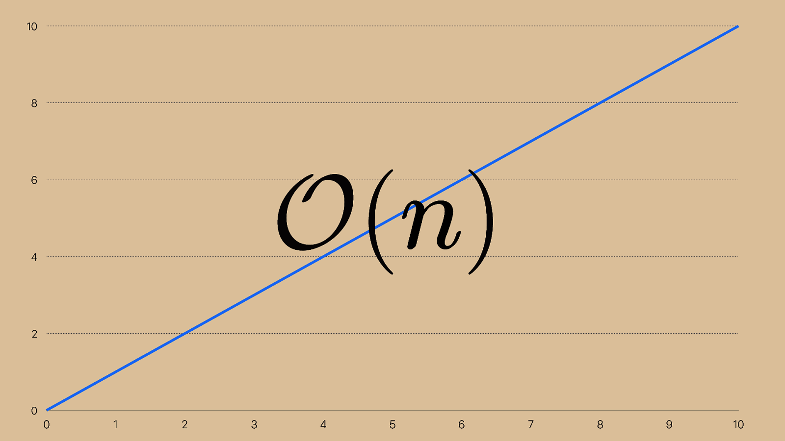
0 2 4 6 8 10 0 1 2 3 4 5 6 7 8 9 10 O ( n ) n That took 15 operations to cut out 16 squares, so it's a linear time complexity algorithm, represented by this notation. It’s read “order of n” and it means linear time. If I wanted to cut out 32 squares, it would take 31 cuts. Even though the number of operations isn't the number of squares, the big O is n because the growth is linear.

You’re probably wondering what the O function is. Here’s a secret: it means nothing. We call it big o notation because we put a big o in front of it, but that’s it.

Ok, let’s look at another algorithm.

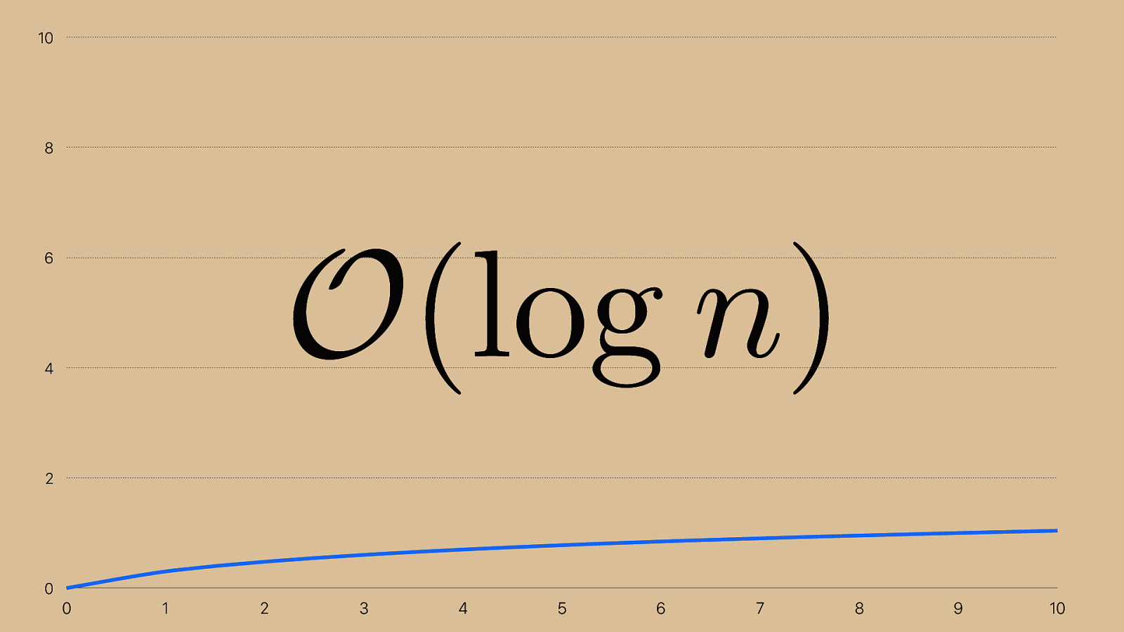
0 2 4 6 8 10 0 1 2 3 4 5 6 7 8 9 10 O (log n ) This new algorithm takes only 4 operations to cut out 16 squares, so it's a O(log n) algorithm. If I wanted to double that to cut out 32 squares, it would take 5 cuts. The difference between logarithmic and linear growth is pretty impressive.

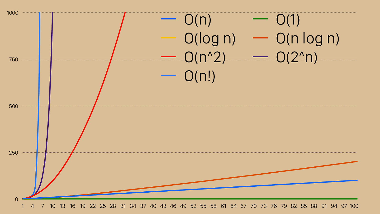
0 250 500 750 1000 1 4 7 10 13 16 19 22 25 28 31 34 37 40 43 46 49 52 55 58 61 64 67 70 73 76 79 82 85 88 91 94 97 100 O(n) O(1) O(log n) O(n log n) O(n^2) O(2^n) O(n!) This is a chart of some of the different common Big O descriptions. On the x axis we have n as it grows, and on the y axis we have time complexity. O(n) and O(log n) are down at the bottom, now orange and yellow. They’re much smaller because I changed the scale from 1:1 on the x and y axis to 10:1. I needed to do that to show the shape of some of these really slow big o representations: n!, 2^n, and n^2. If you draw an imaginary line diagonally across this chart, you basically want to avoid any of the big o values above it and shoot for the big o values below it.

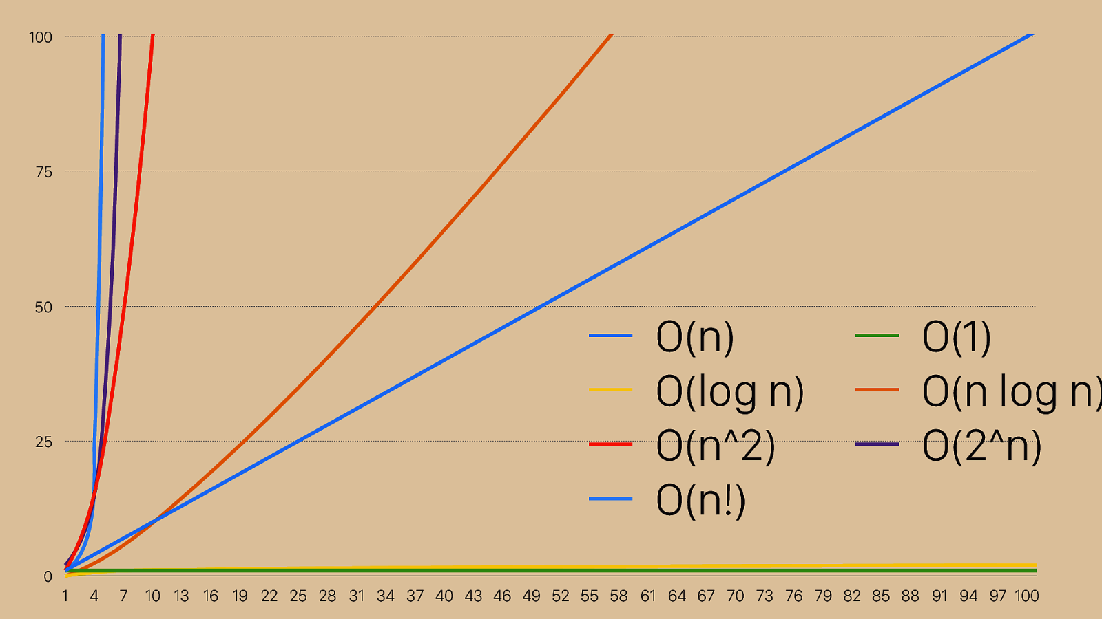
0 25 50 75 100 1 4 7 10 13 16 19 22 25 28 31 34 37 40 43 46 49 52 55 58 61 64 67 70 73 76 79 82 85 88 91 94 97 100 O(n) O(1) O(log n) O(n log n) O(n^2) O(2^n) O(n!) If we switch back to our 1:1 ratio, you can see that even these more performant options have a lot of variation. That’s why O(n) was so much more complicated than O(log n).

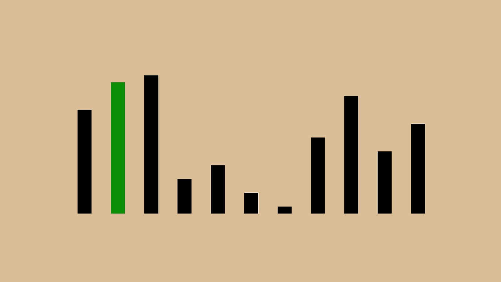
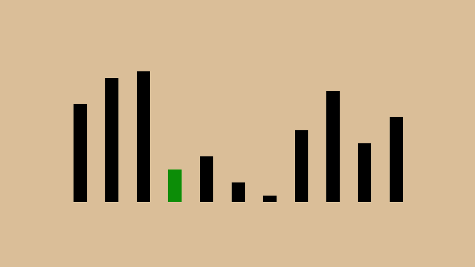
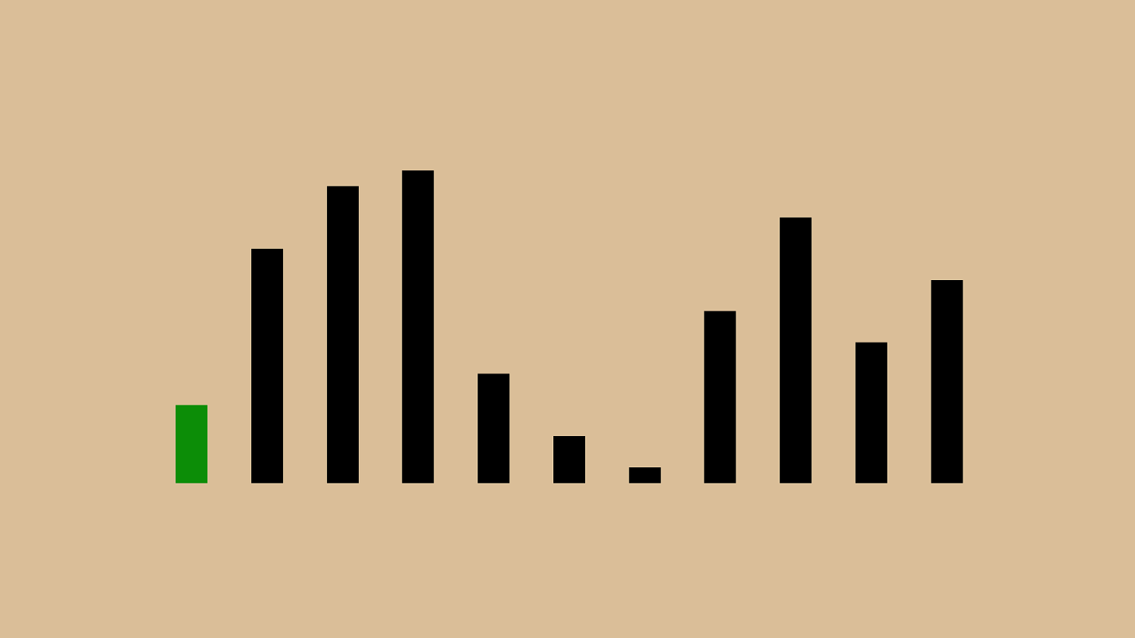
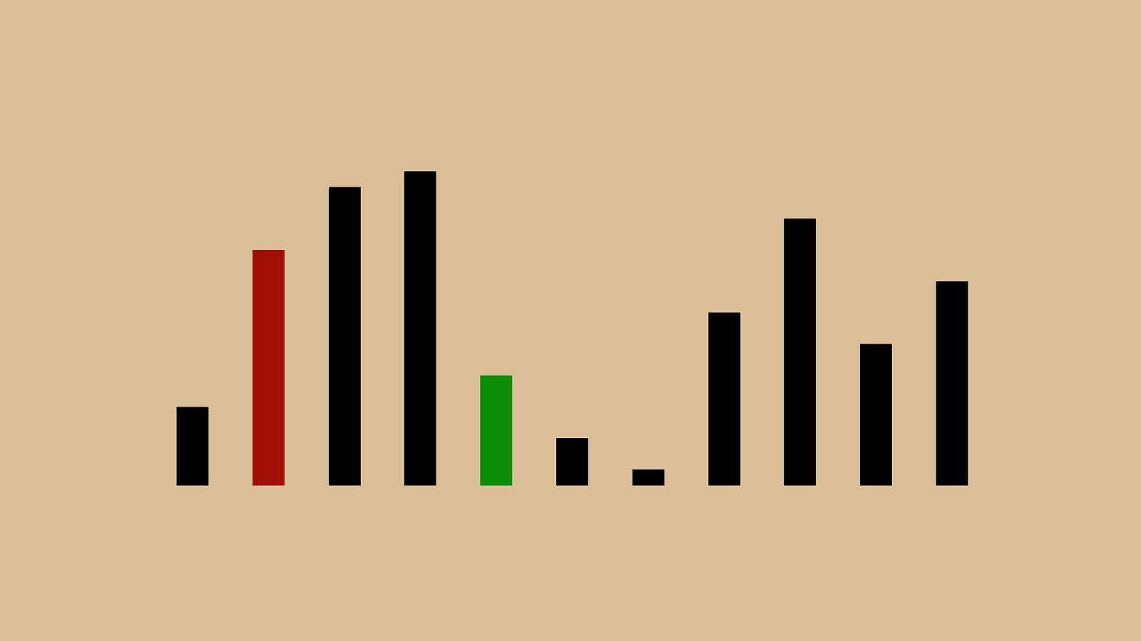
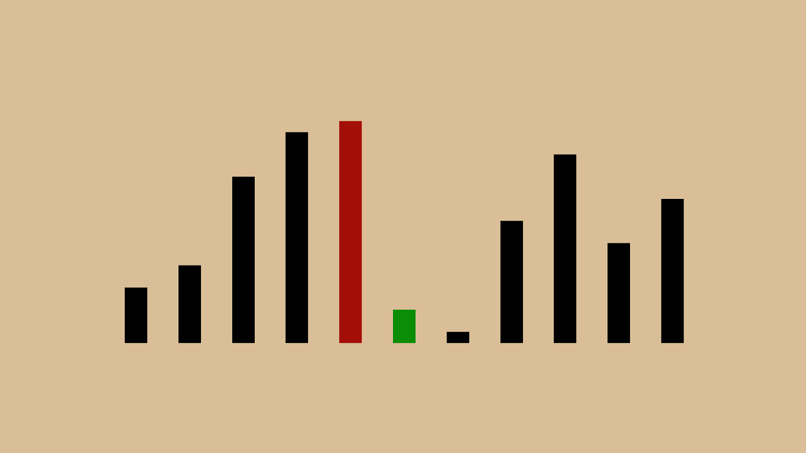
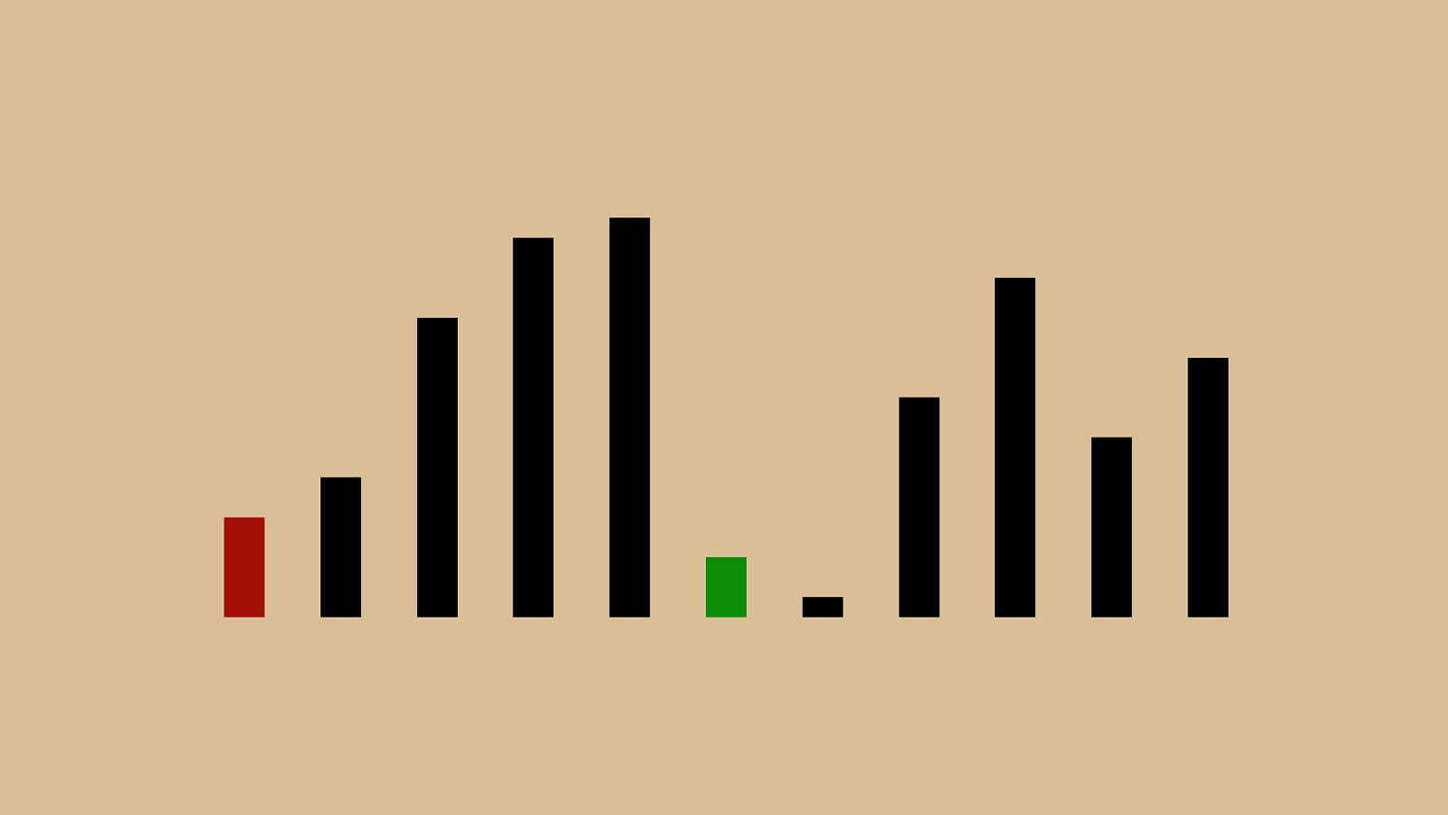
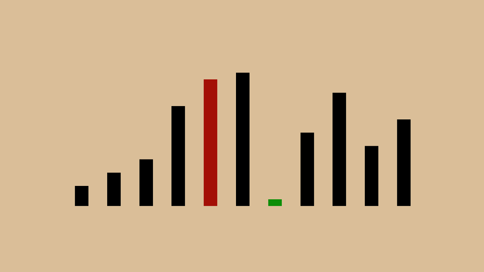
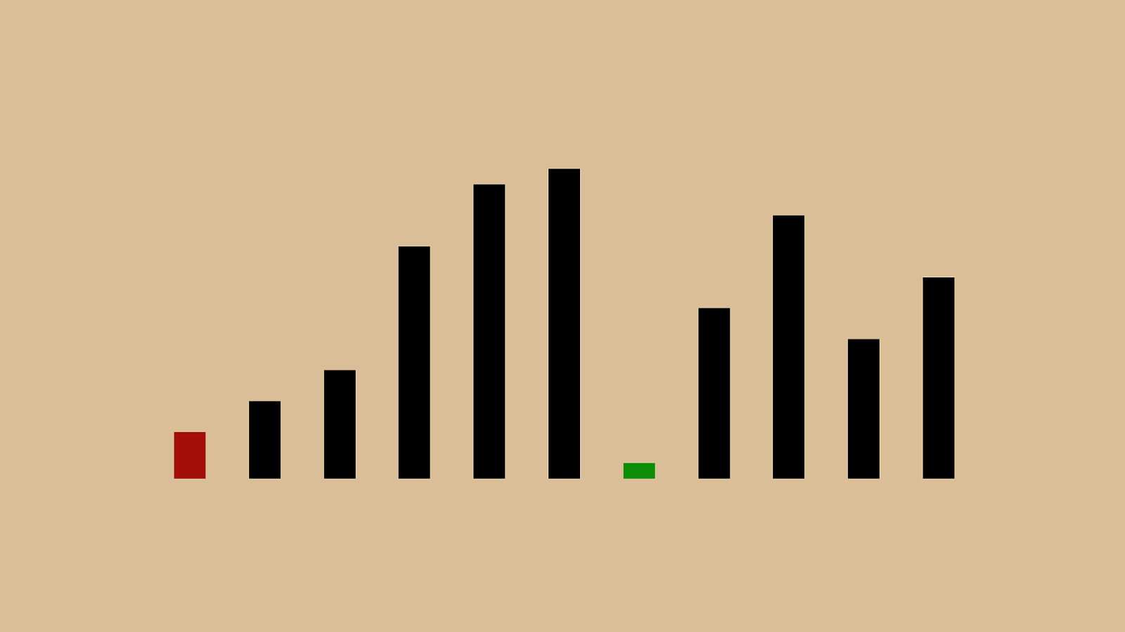
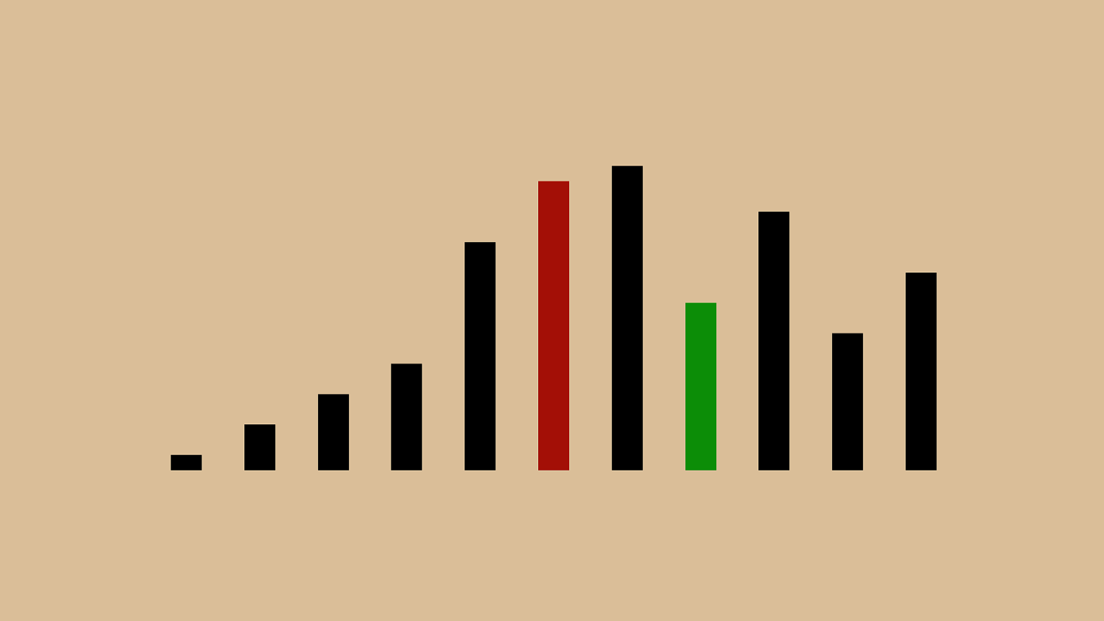
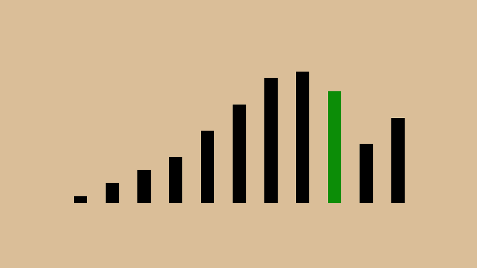
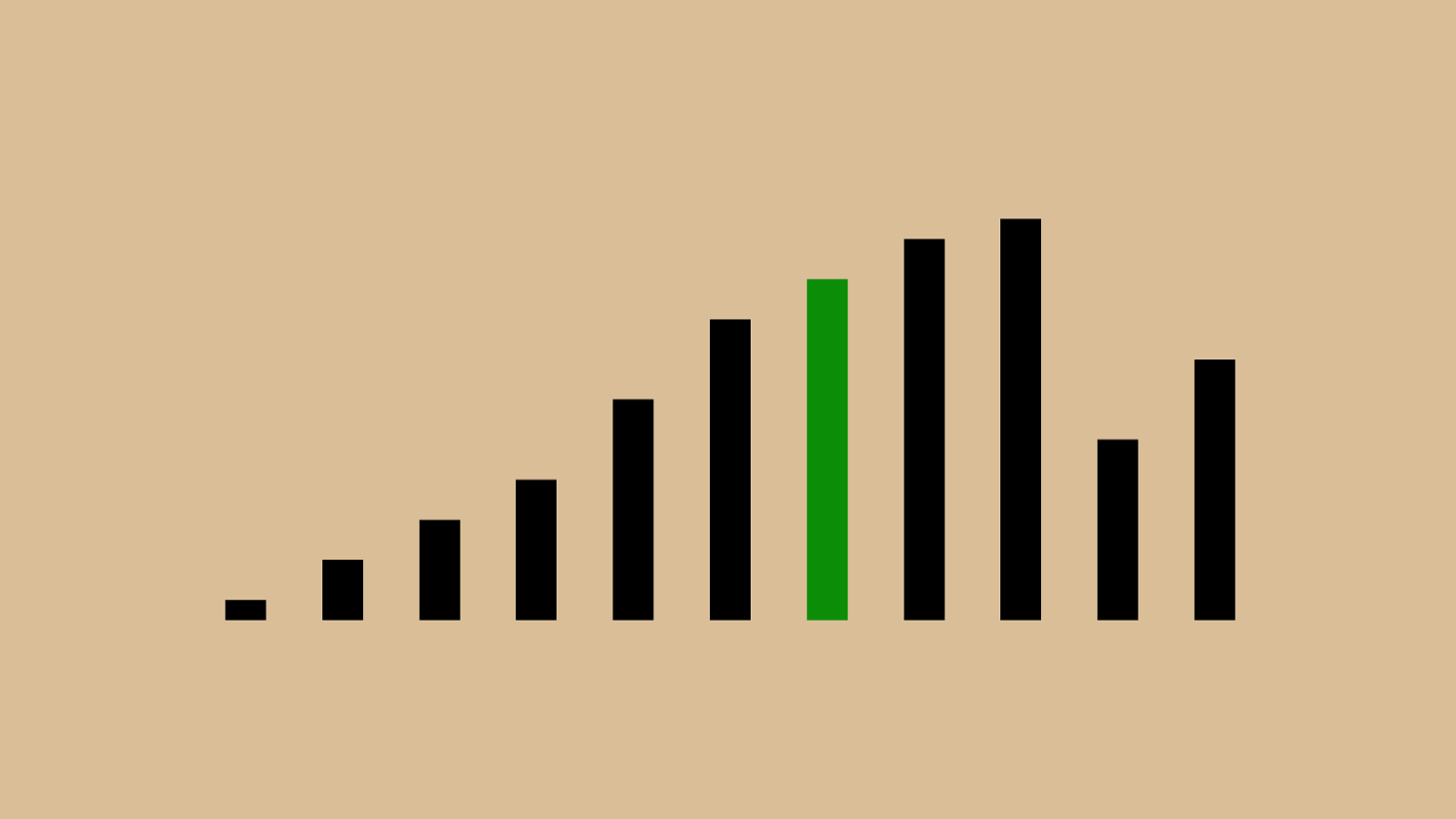
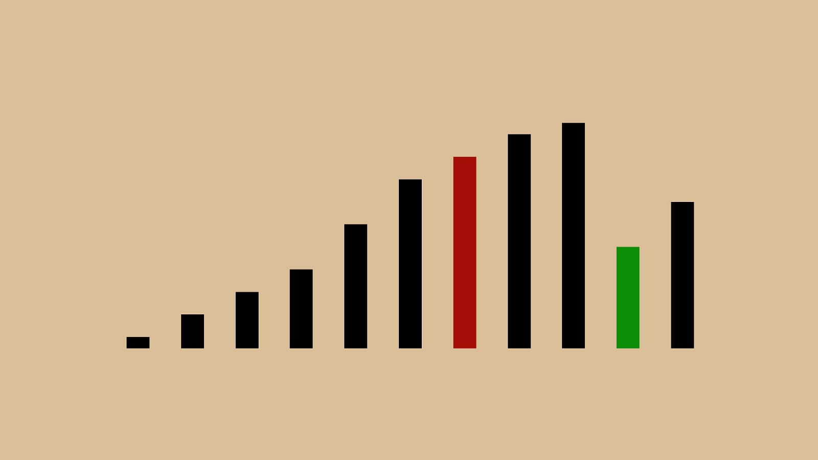
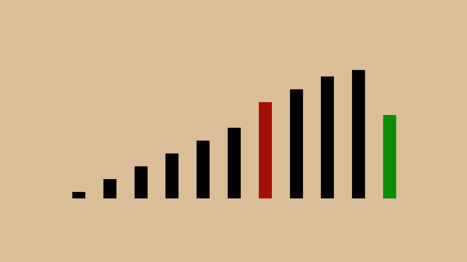
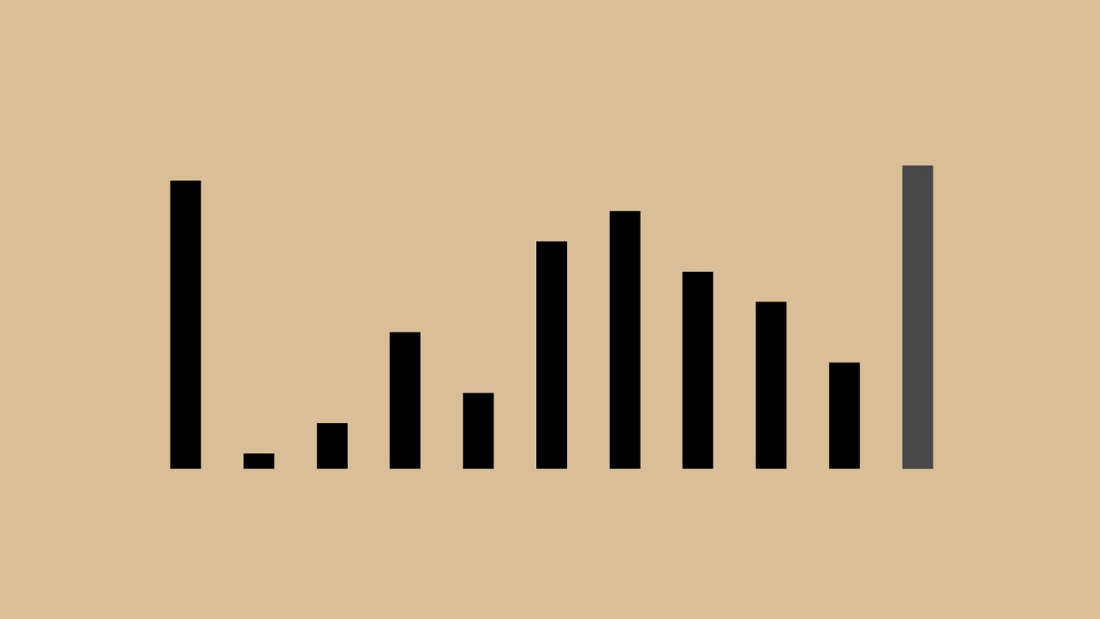
When do you update a user record?

When do you update a user record? O ( n log n )

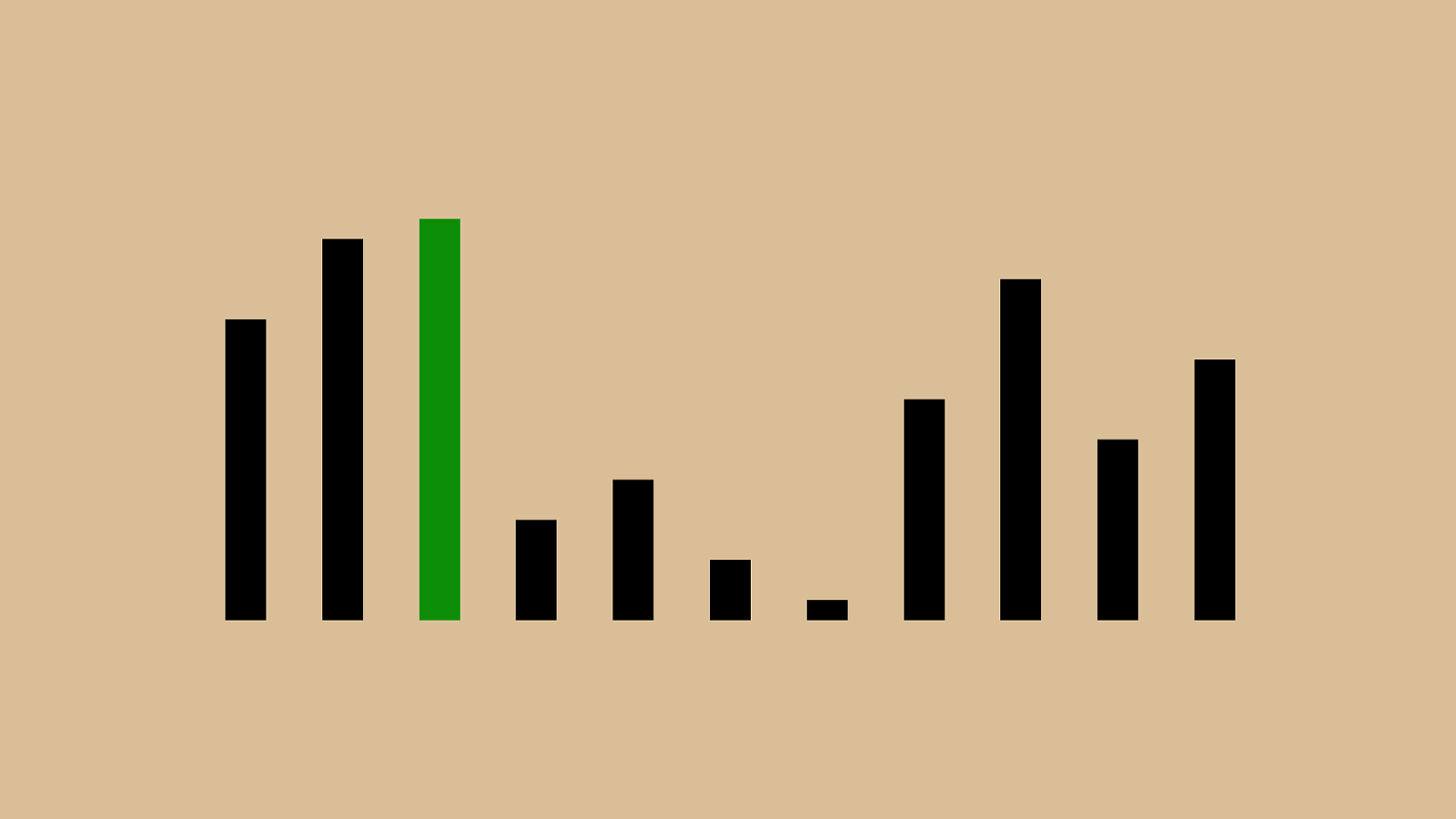
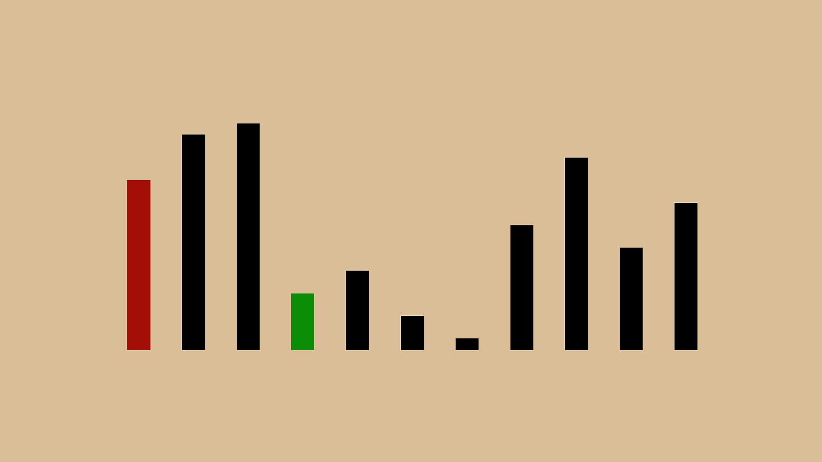
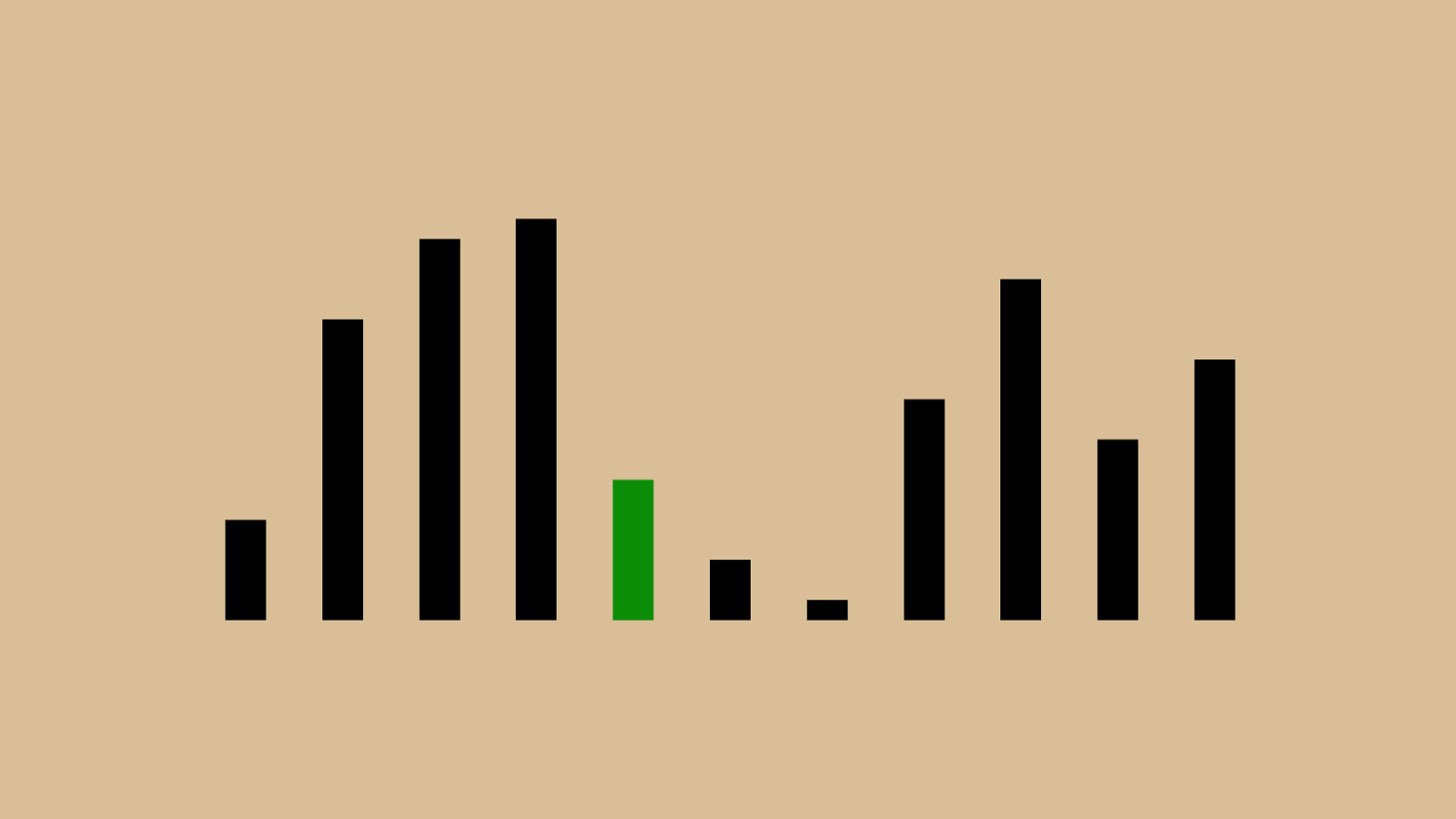
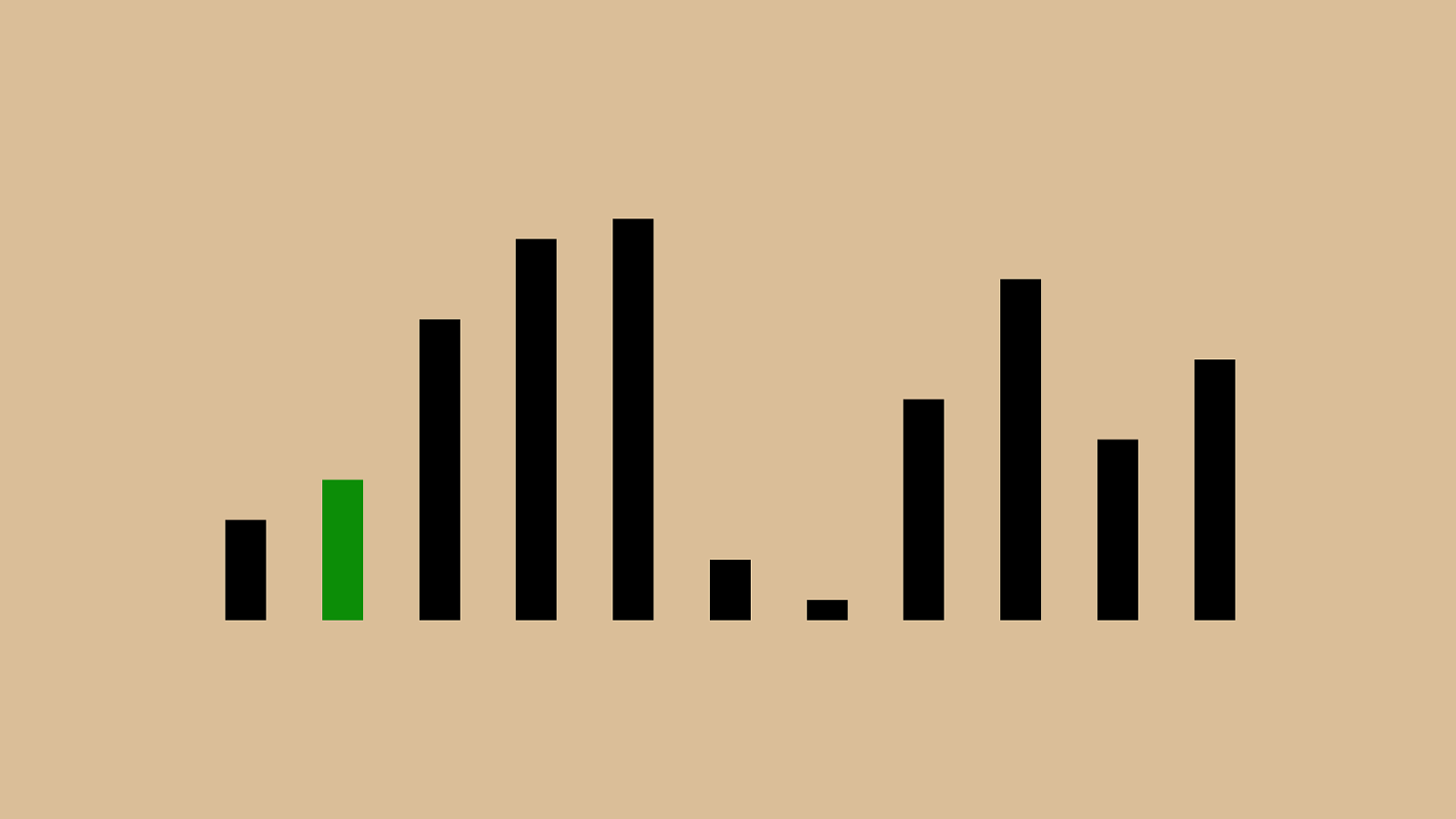
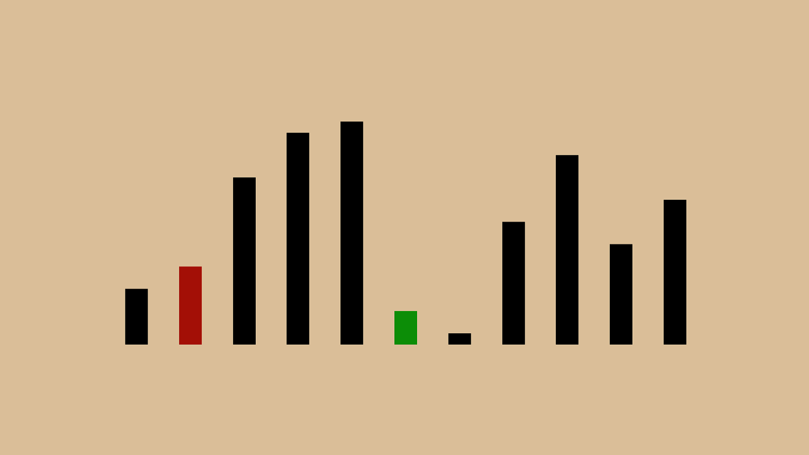
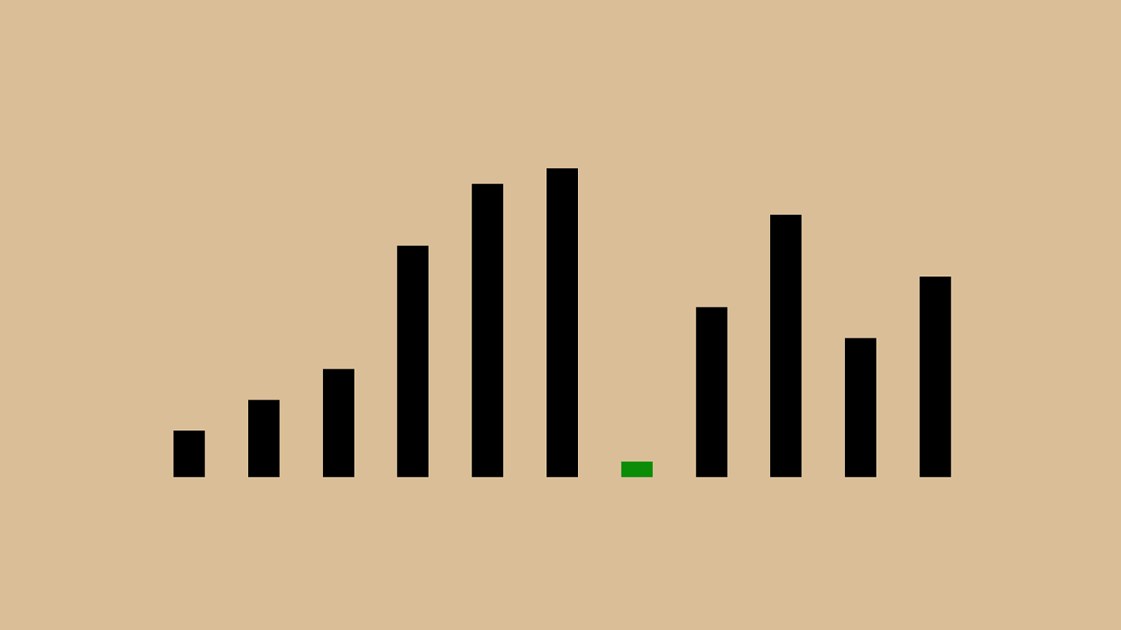
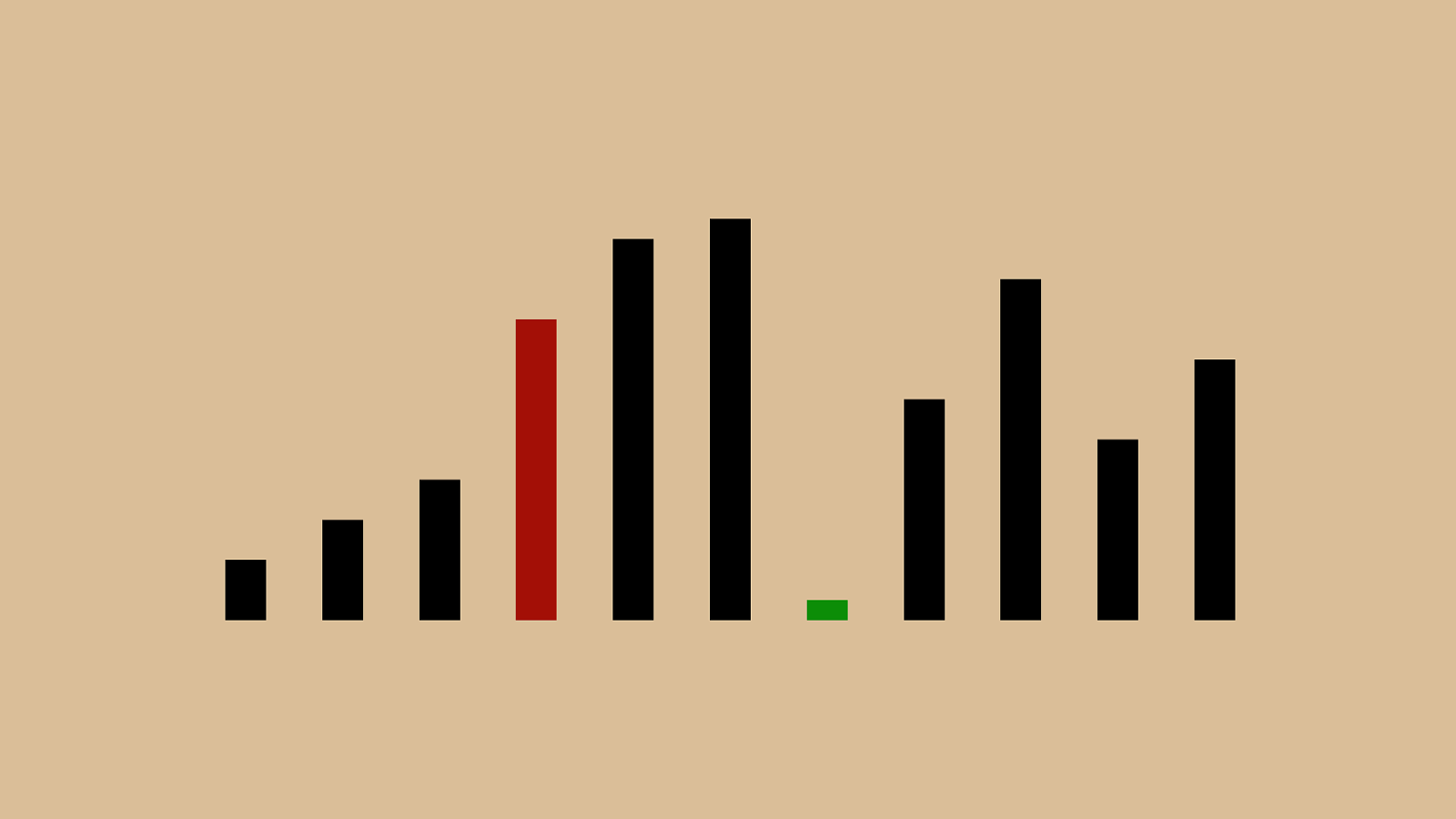
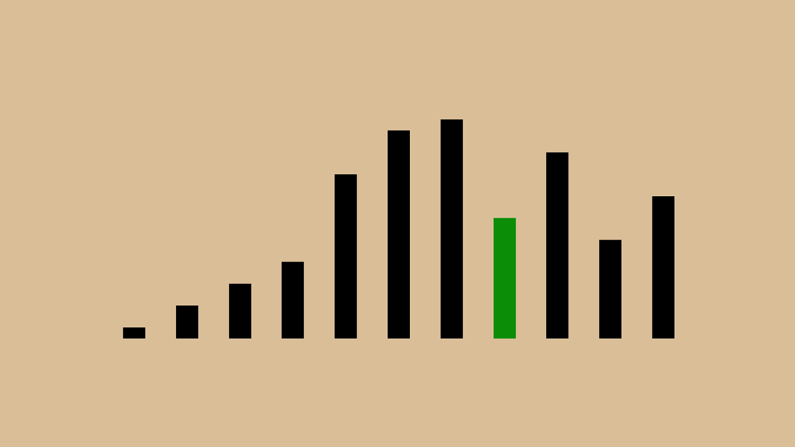
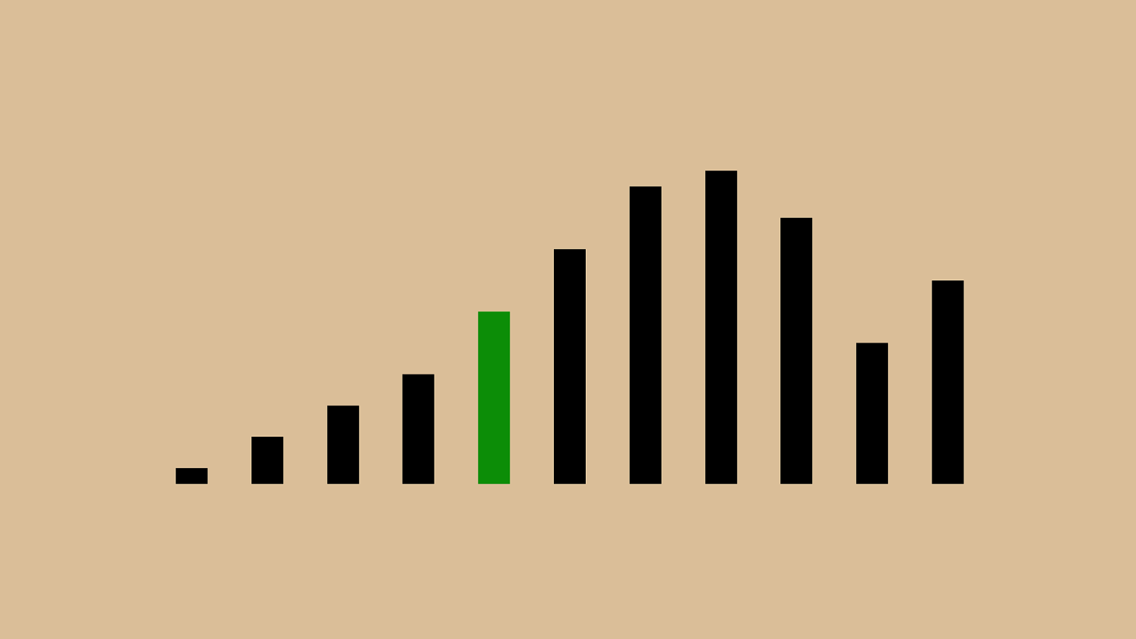
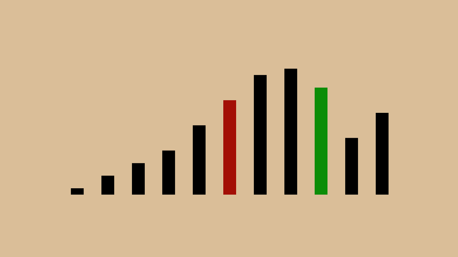
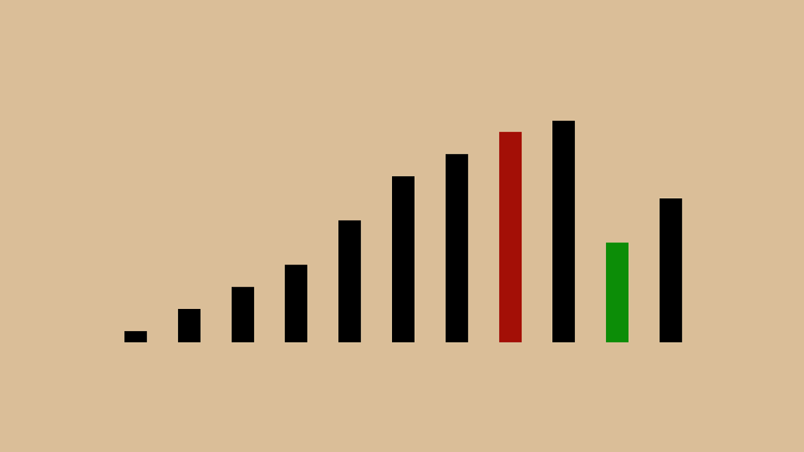
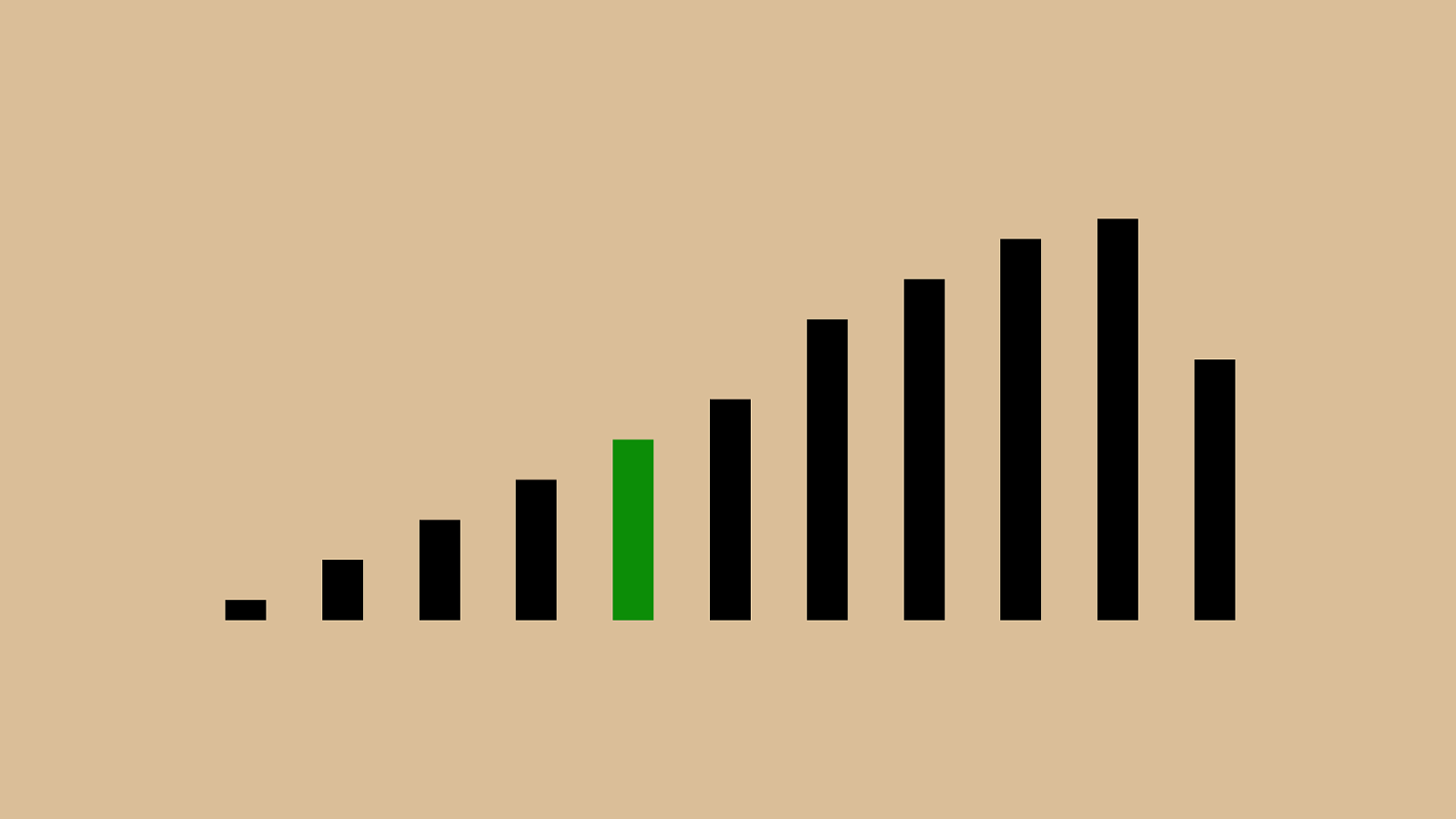
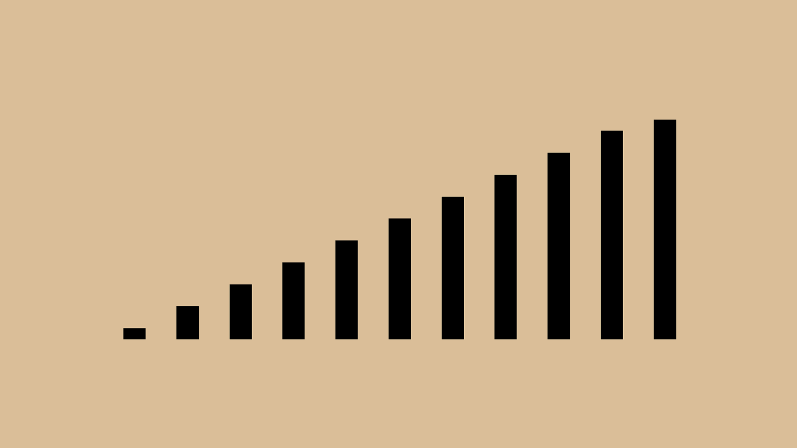
If you understood everything

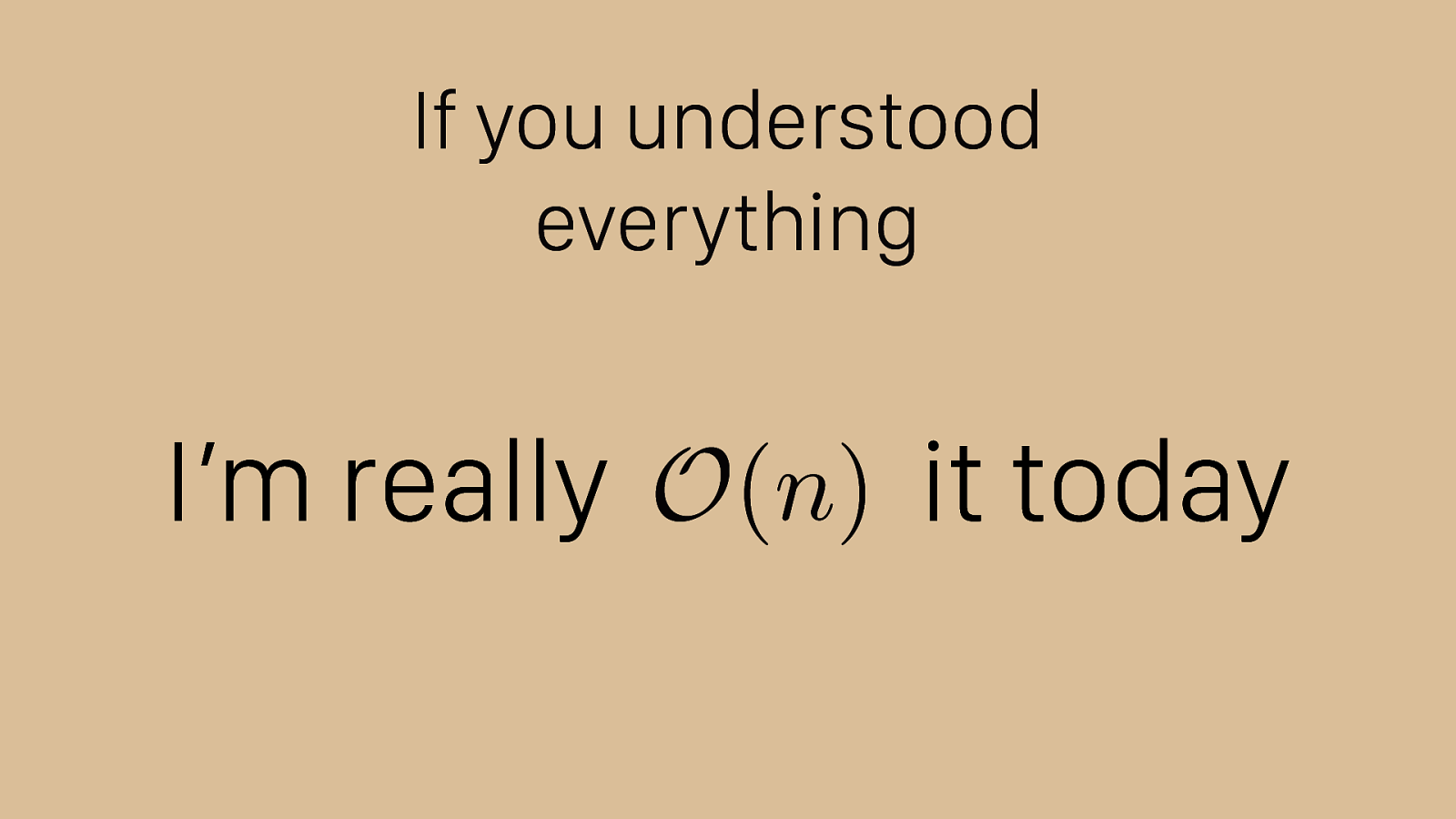
If you understood everything I’m really it today O ( n )

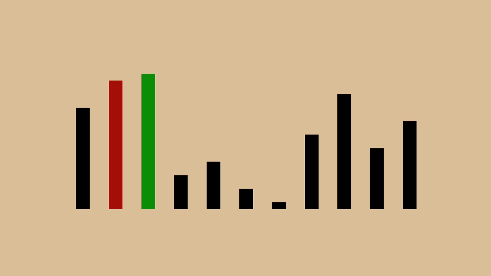
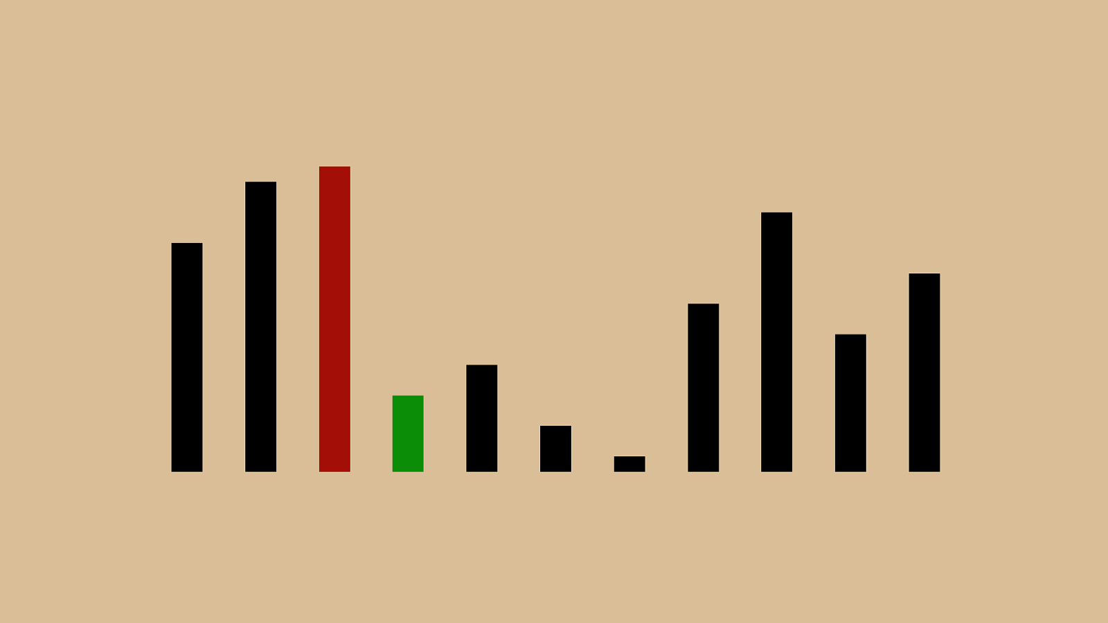
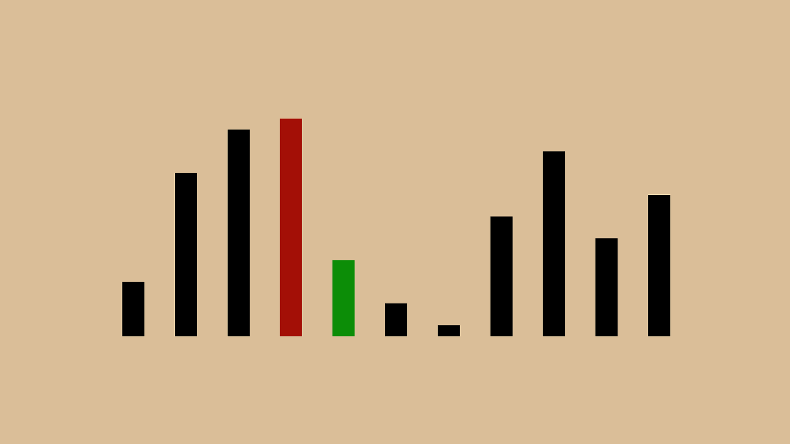
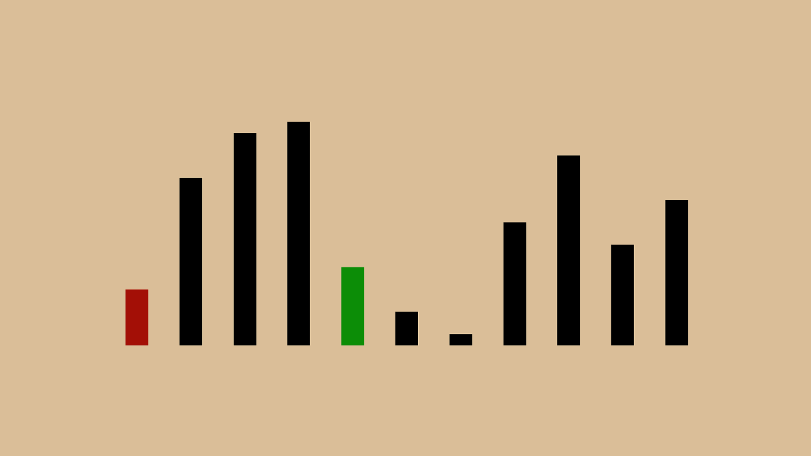
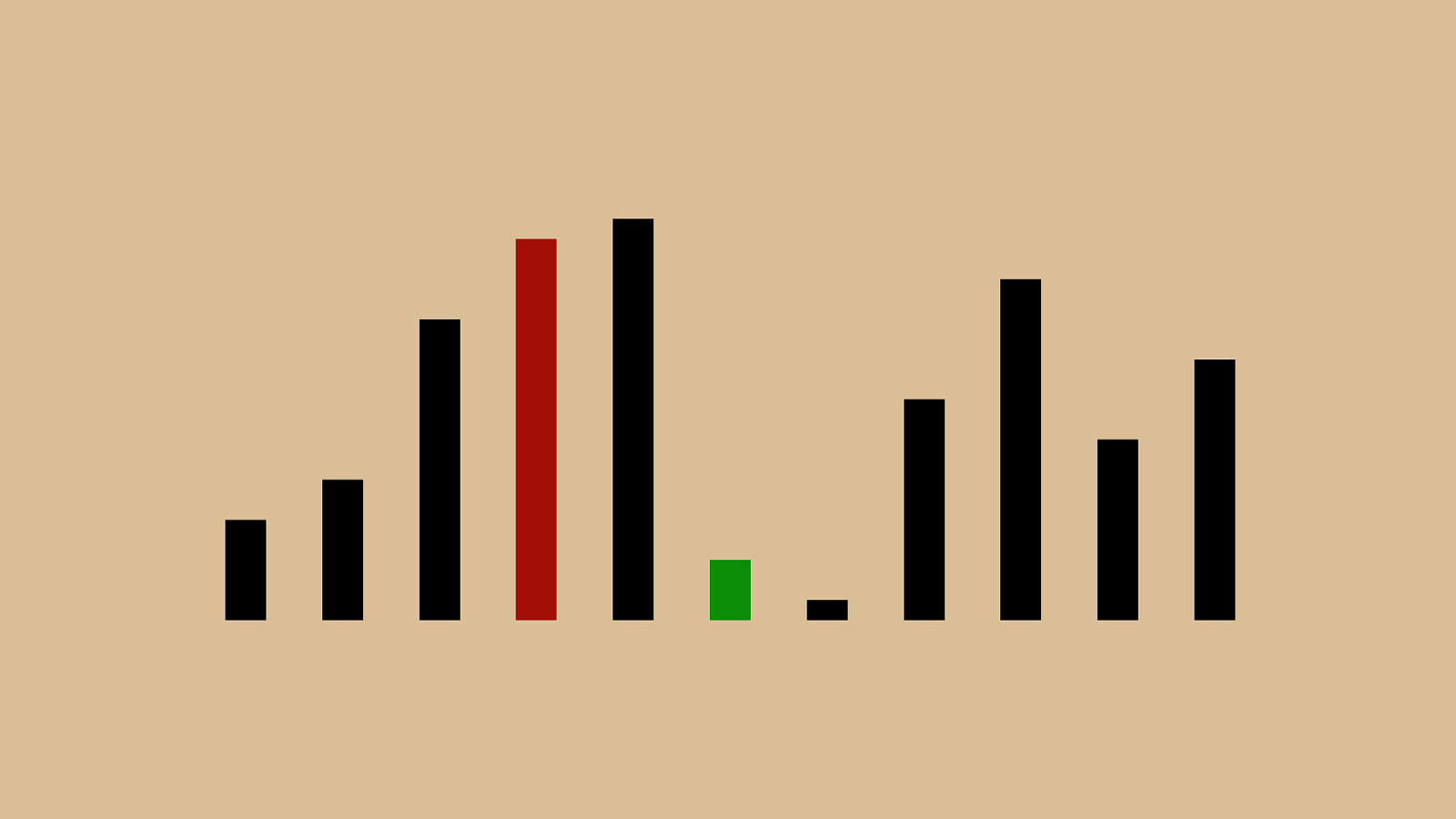
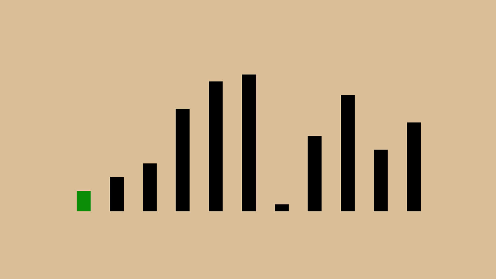
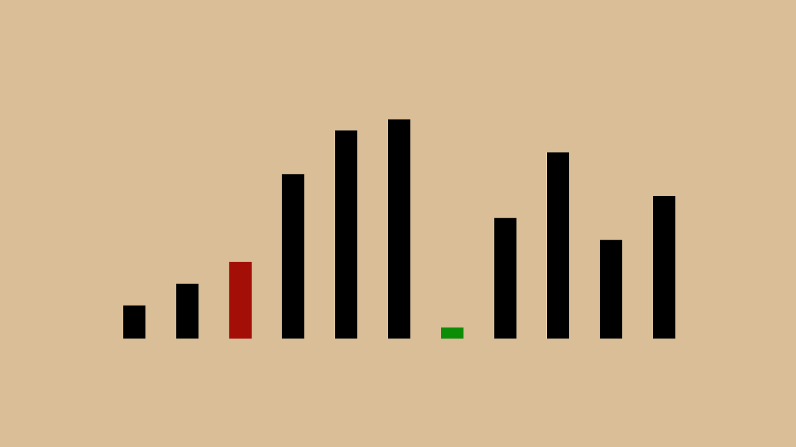
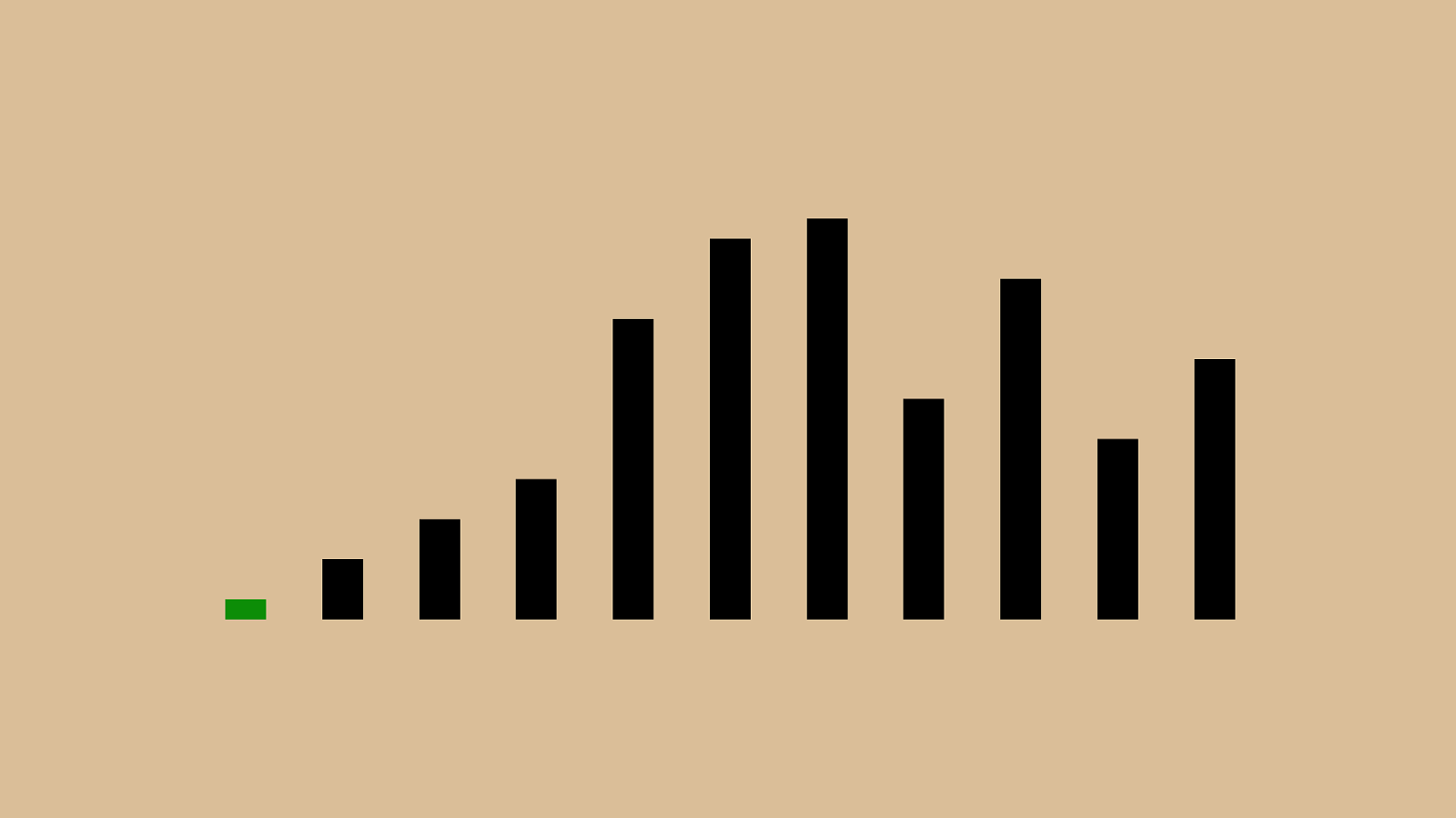
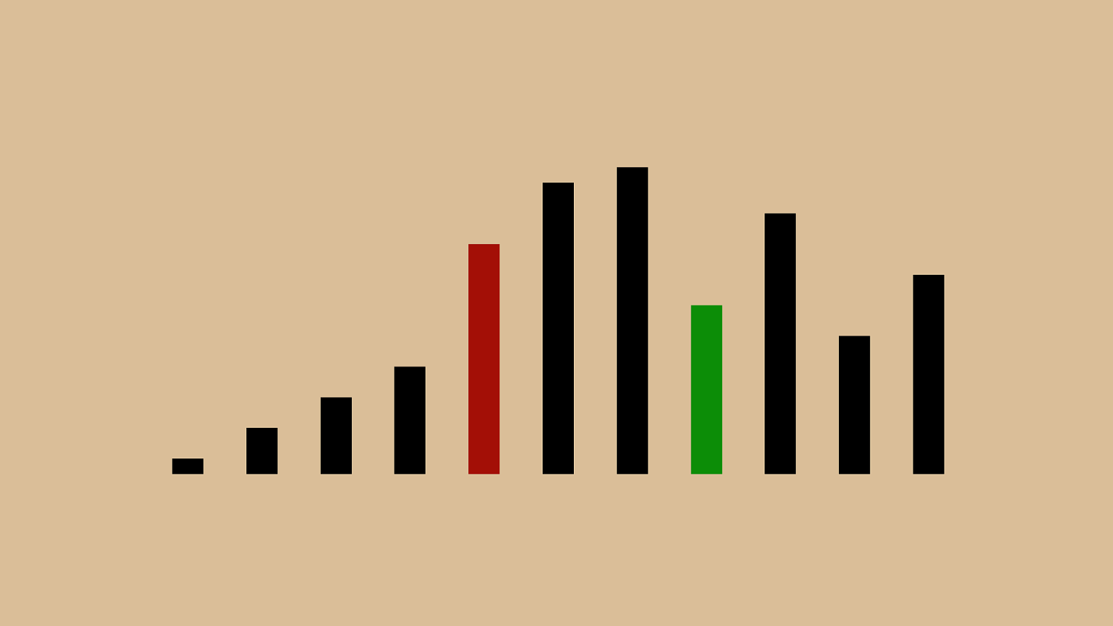
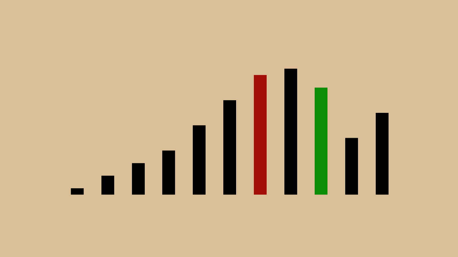
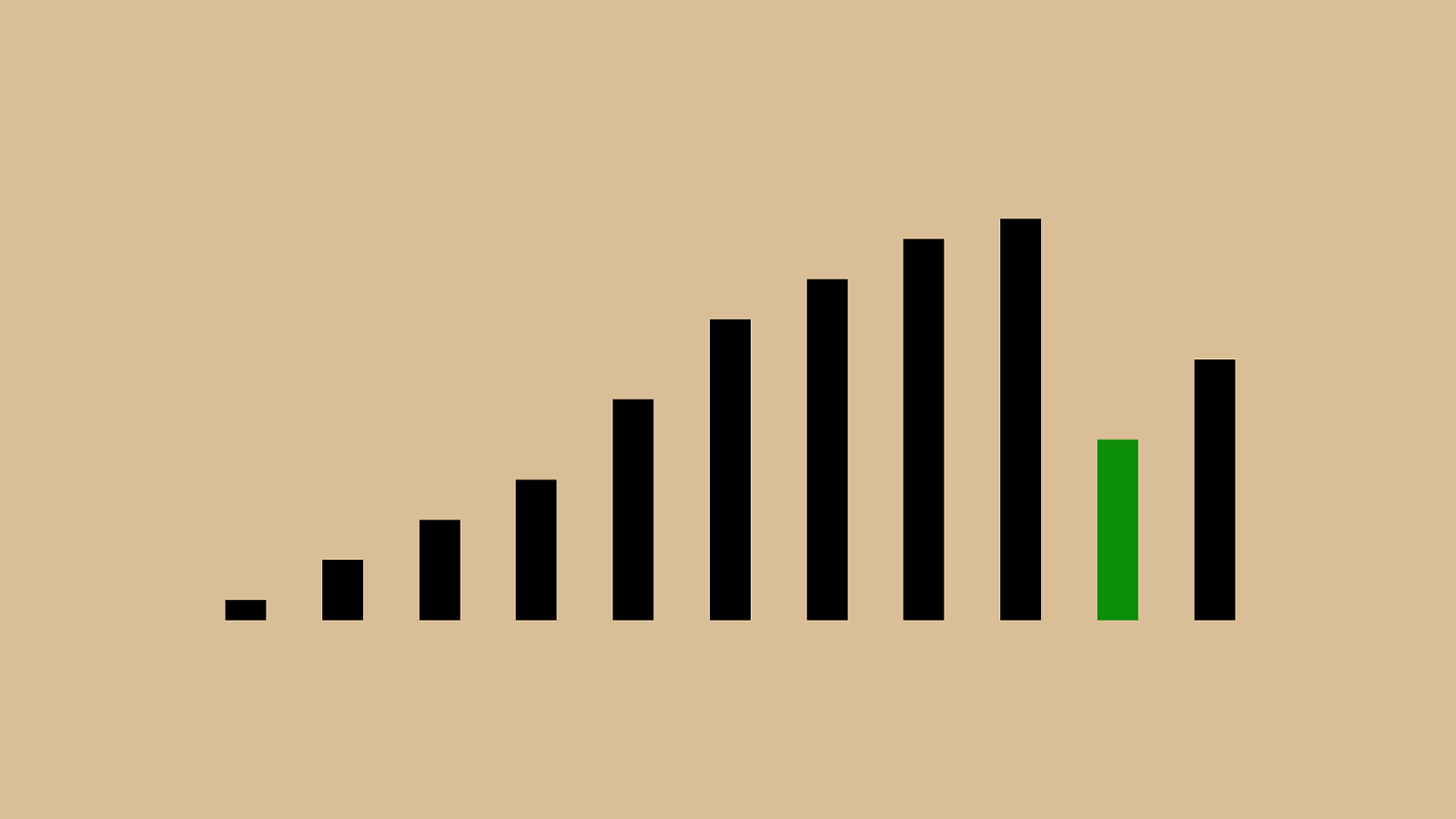
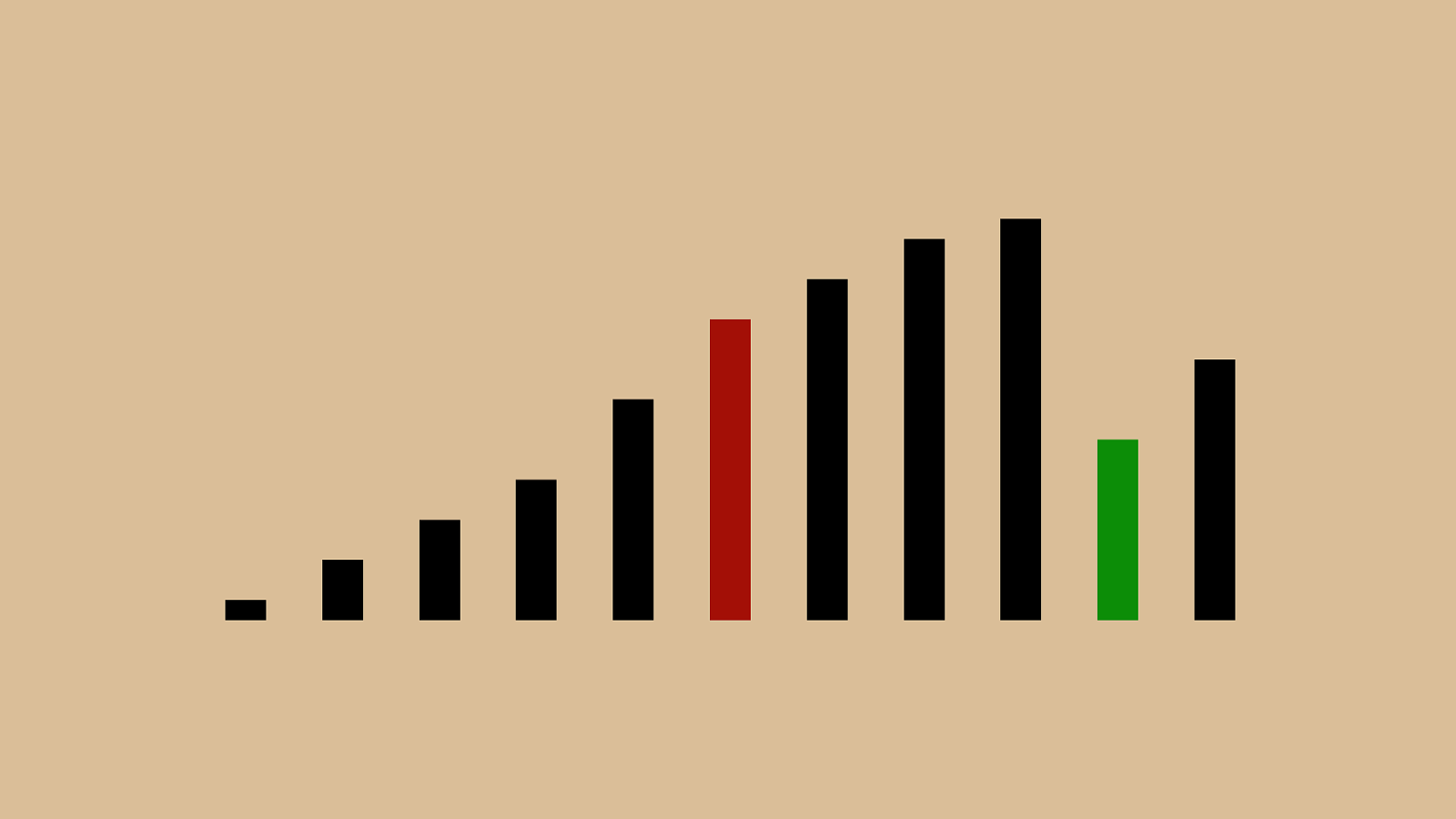
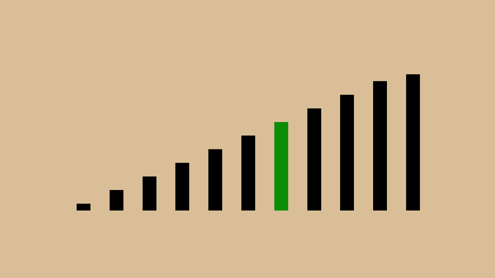
How do you debug an app?

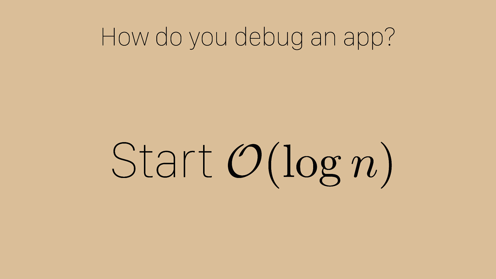
How do you debug an app? Start O (log n )

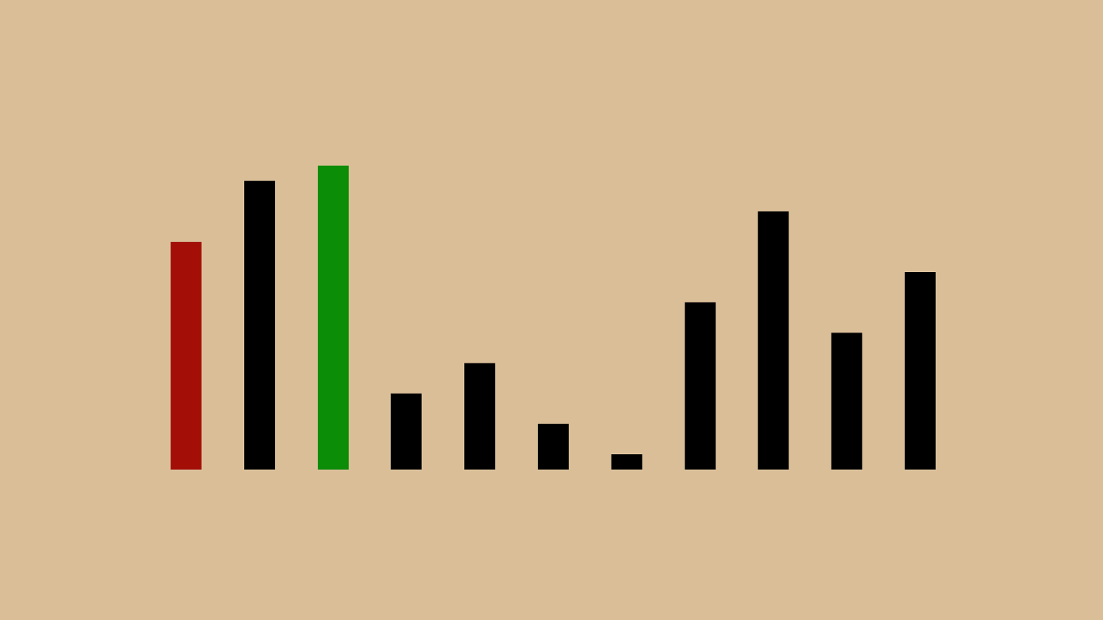
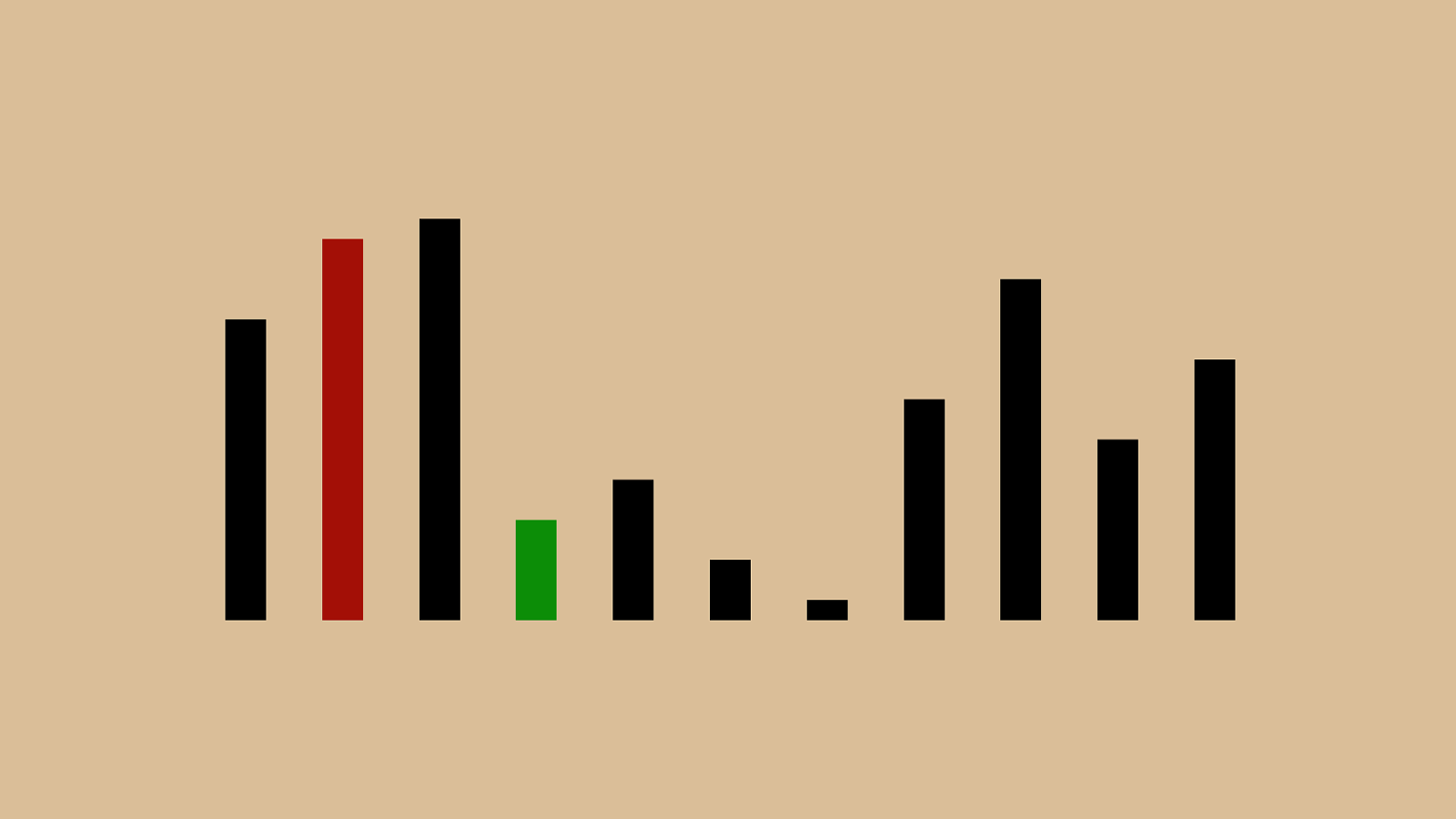
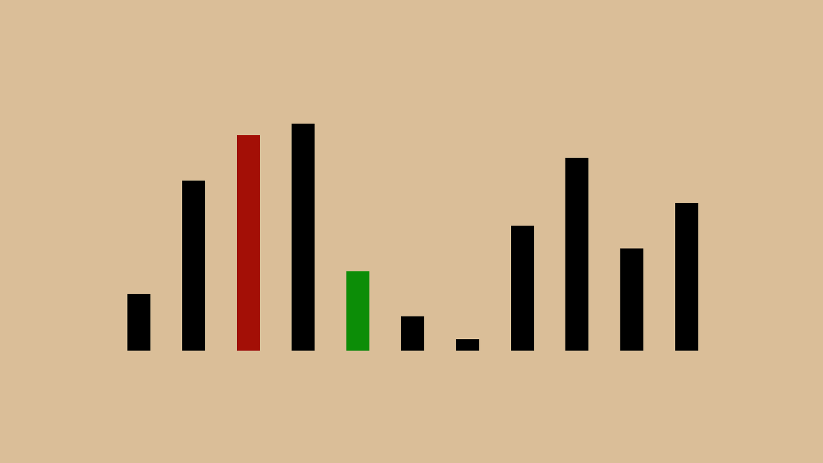
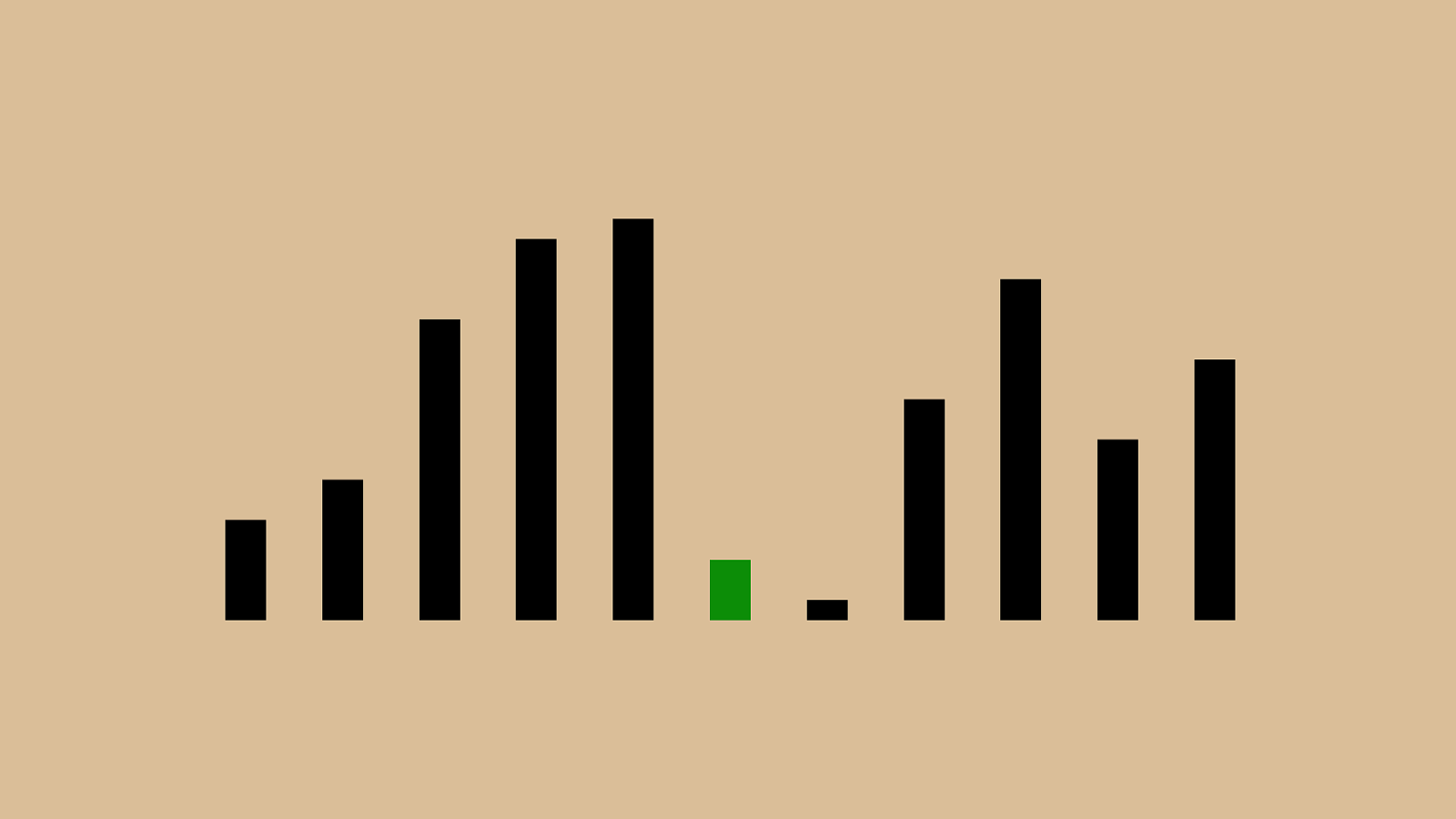
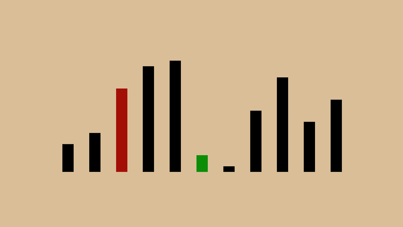
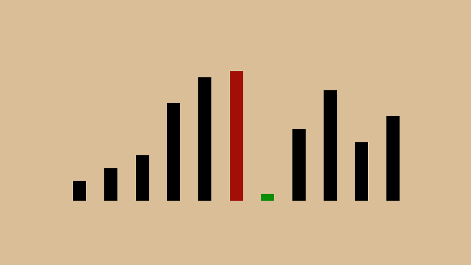
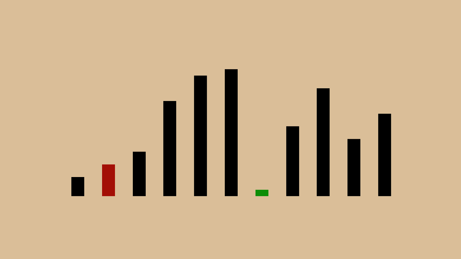
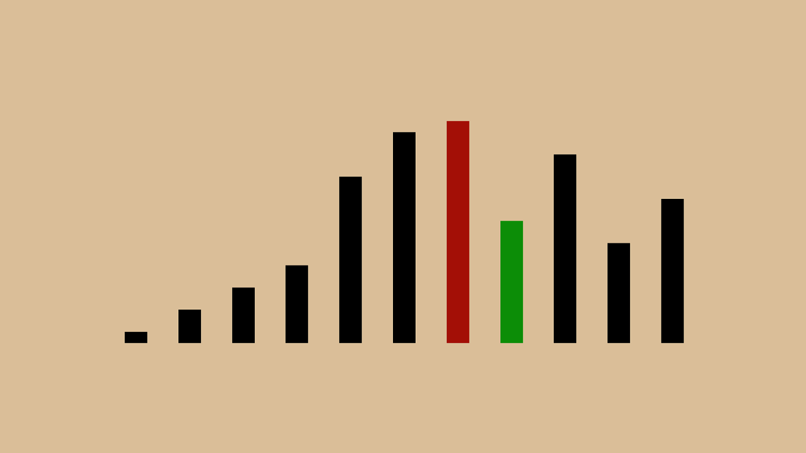
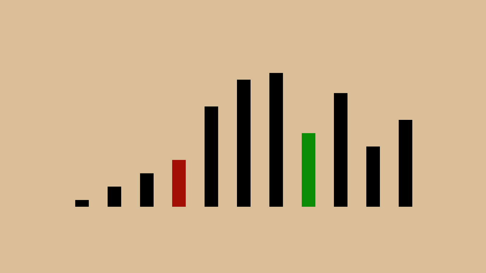
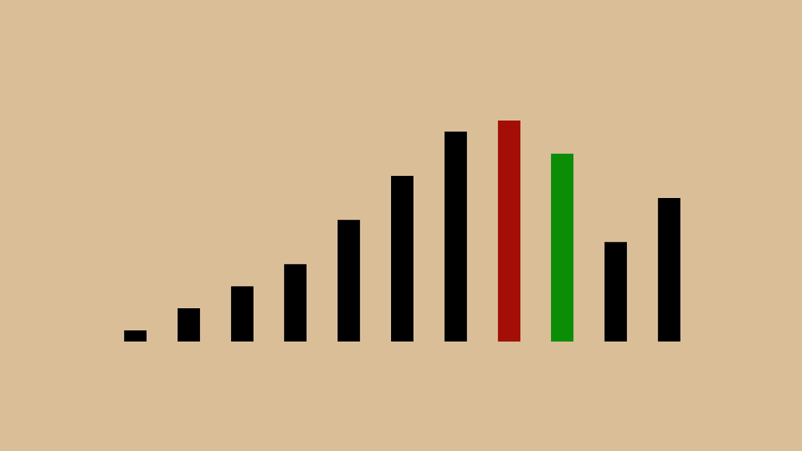
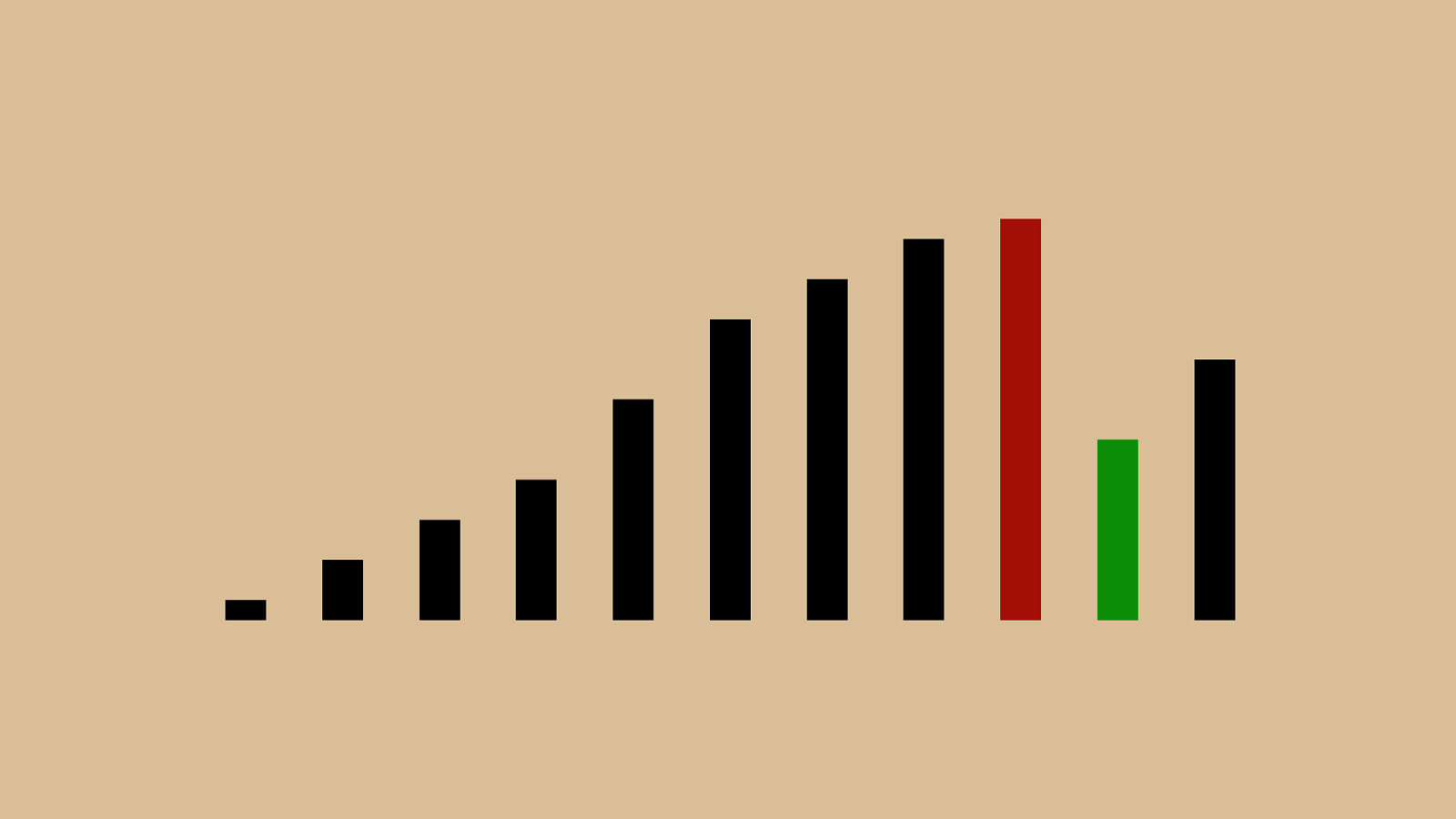
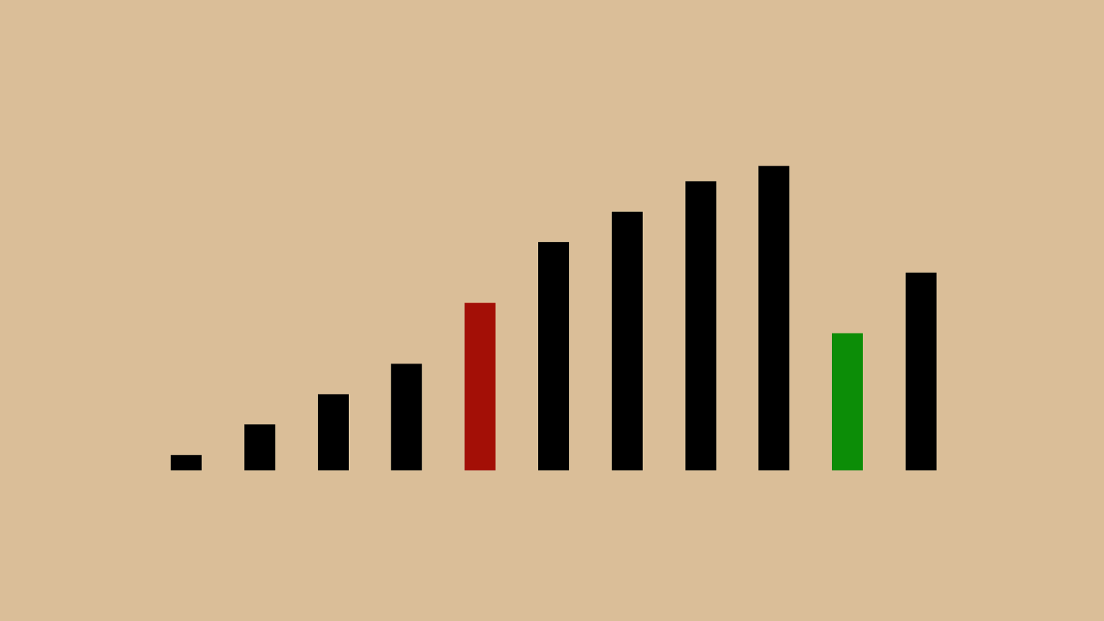
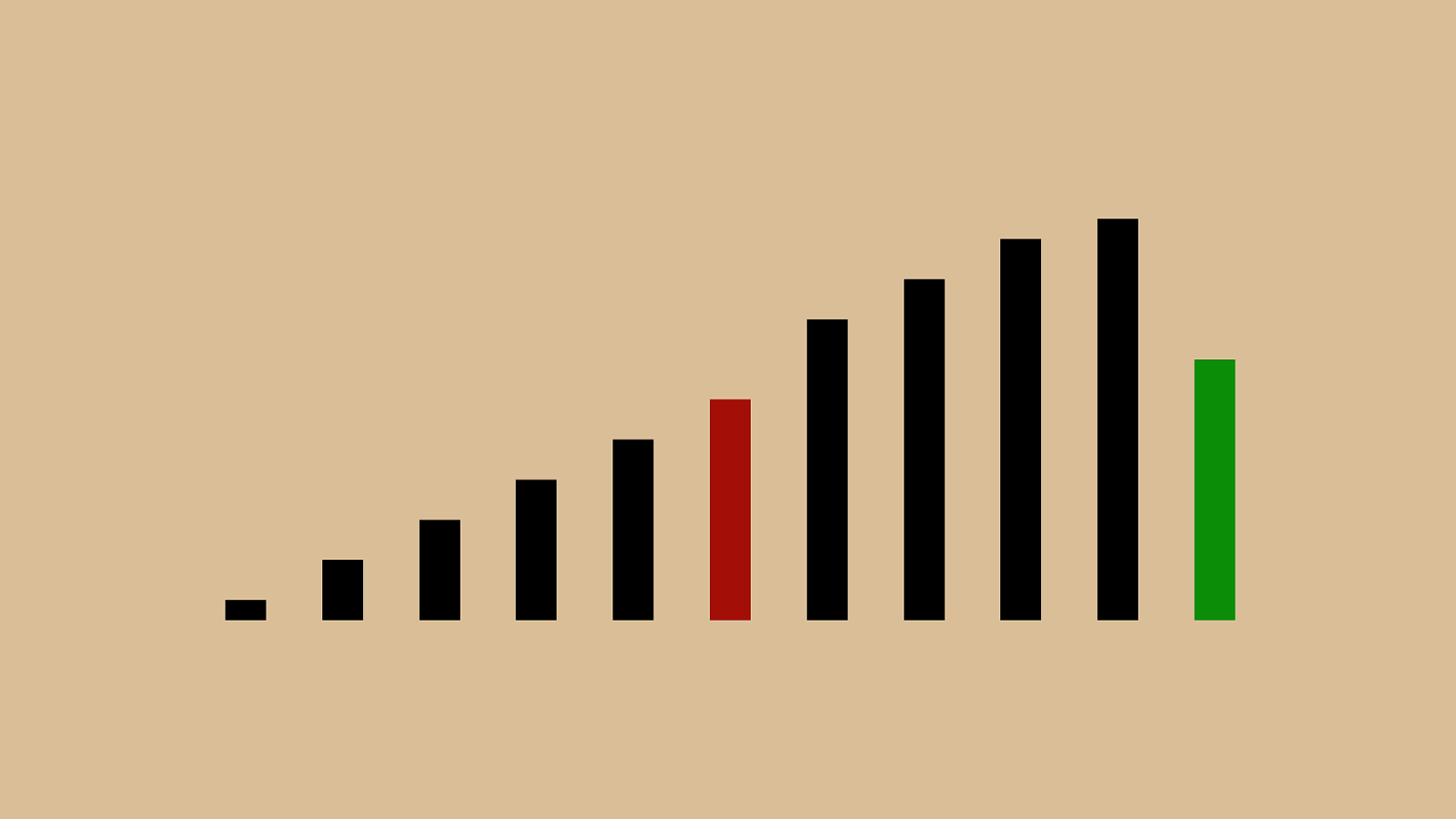
What happens when you buy something?

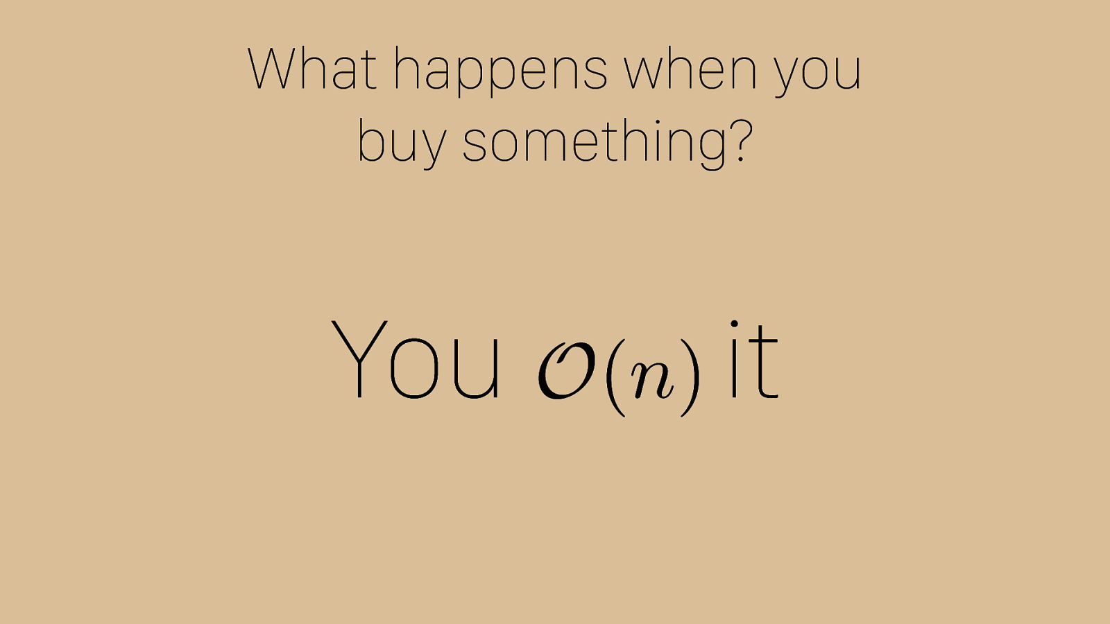
What happens when you buy something? Yo u i t O ( n )

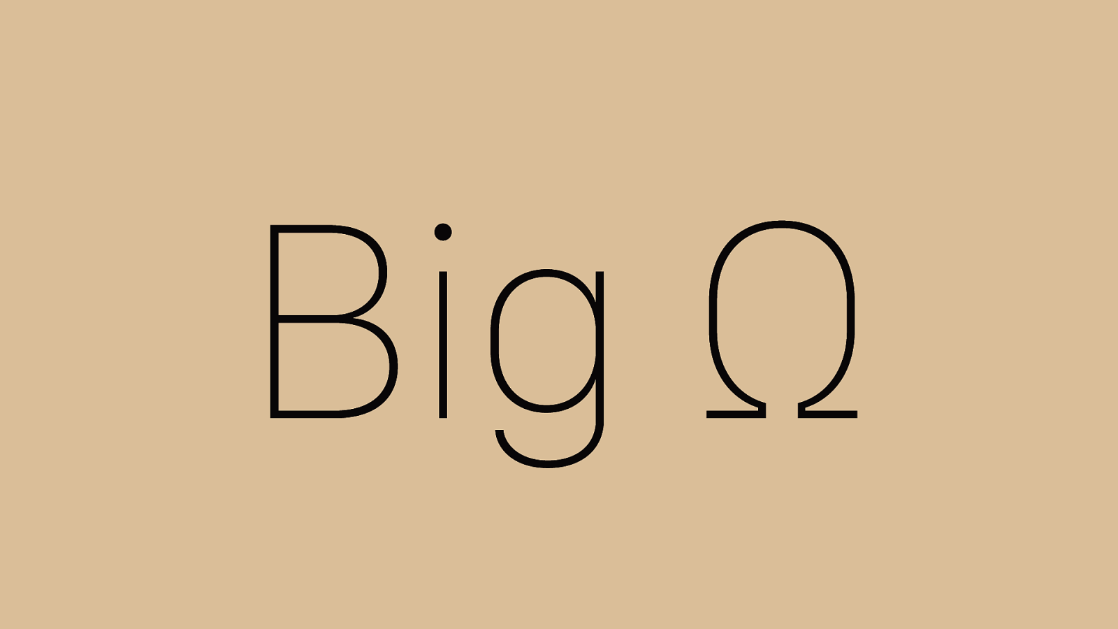
Big Ω We’re also going to talk about Big Omega. This one’s easy. It’s the same as Big O, but instead of talking about worst case performance, it means best case performance. That’s why it has these tails here at the lower part of the symbol, since it’s the lower bound for how fast an algorithm is.

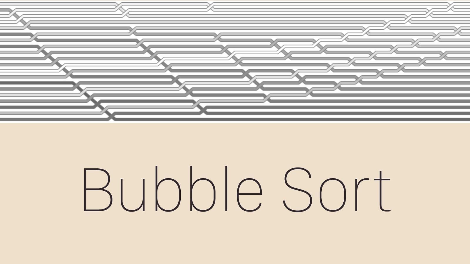
Bubble Sort The bubble sort algorithm is nice and simple, so it’s a great place to jump into explaining sorting algorithms.

The algorithm is: consider each pair of elements. If they’re in the wrong order, swap them. Then move one over and repeat. Keep doing that until you hit the end of the set, then start over. Remember where you left the biggest thing you found, and don’t go past it. If you go through an entire iteration and no changes are made, you’re sorted.

42 9001 5.1 pi e

2 ) n O ( Bubble sort works on O(n^2) time.

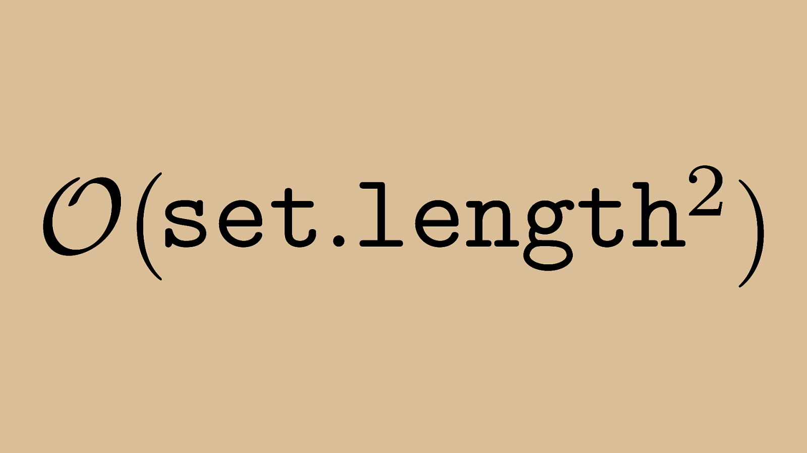
2 ) O ( set . length For the purposes of sorting algorithms, “n” is the length of the set.

2 ) n O ( Bubble sort operates in n^2 time because it compares every element to every other element in the worst case. Even though we have some optimizations so that you’re not comparing every single element, when we’re stating an algorithm’s complexity we still say n^2.

For bubble sort, O(n^2) is also the average case complexity (such as on a randomized array).

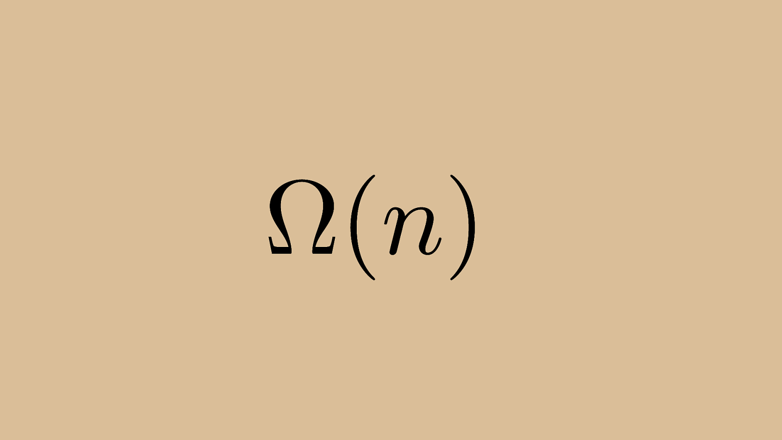
⌦ ( n ) It has Big Omega (or lower bound / best case) time of n, which means that for its best case, which for Bubble Sort is a sorted set, it takes only “n” comparison operations to confirm that we are sorted.

0 250 500 750 1000 1 4 7 10 13 16 19 22 25 28 31 34 37 40 43 46 49 52 55 58 61 64 67 70 73 76 79 82 85 88 91 94 97 100 O(n) O(1) O(log n) O(n log n) O(n^2) O(2^n) O(n!) As we saw before, n^2 isn’t very good. It’s that Rad line there, and in this case bigger is worse, because it means number of operations and usually also time taken. What we want is to be in one of these four smaller lines, O(n log n), O(n), or ideally O(log n) or O(1). O(1) only works in a perfect world where your sorting algorithm is to return the sorted set you were asked to sort.

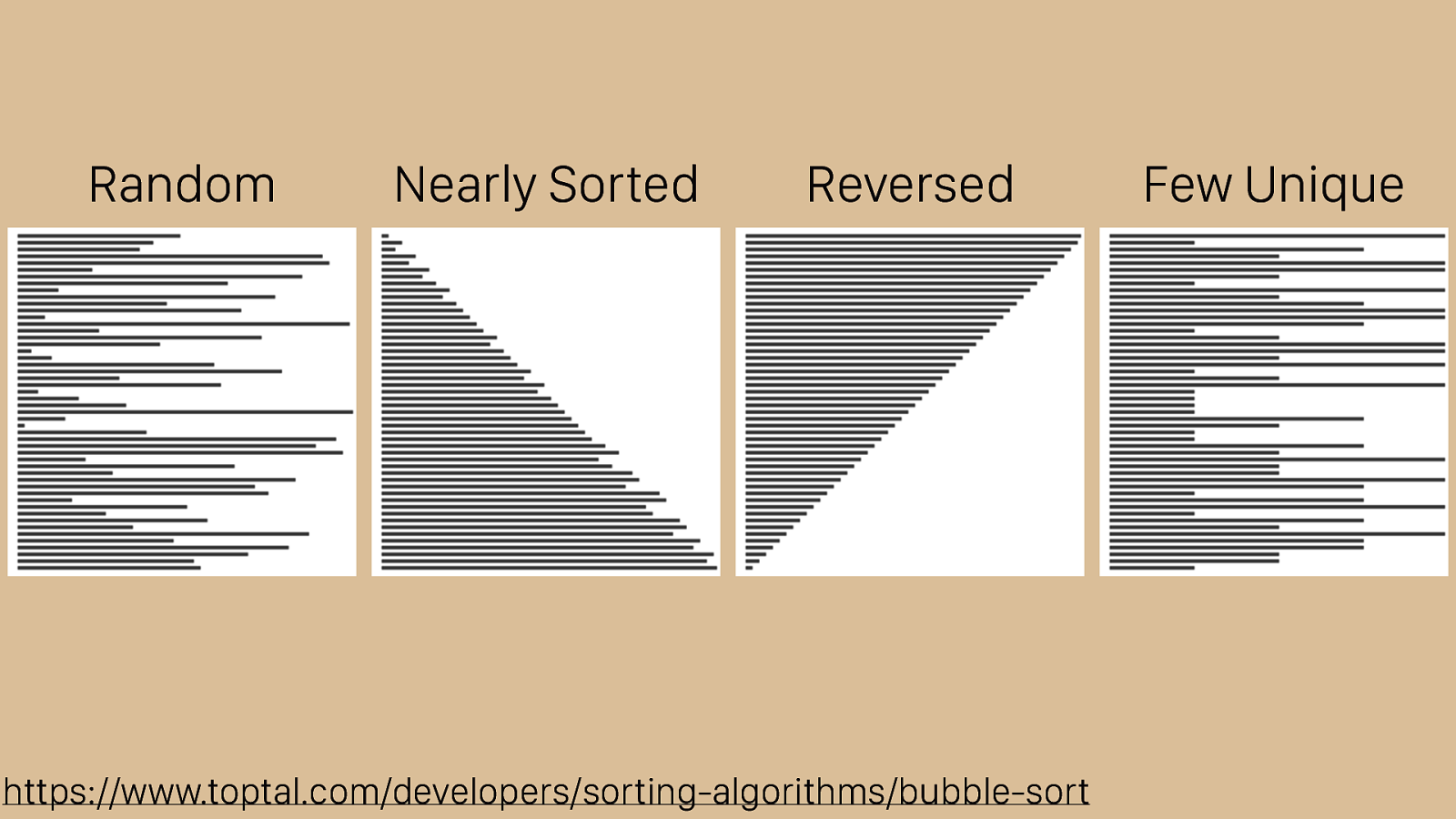
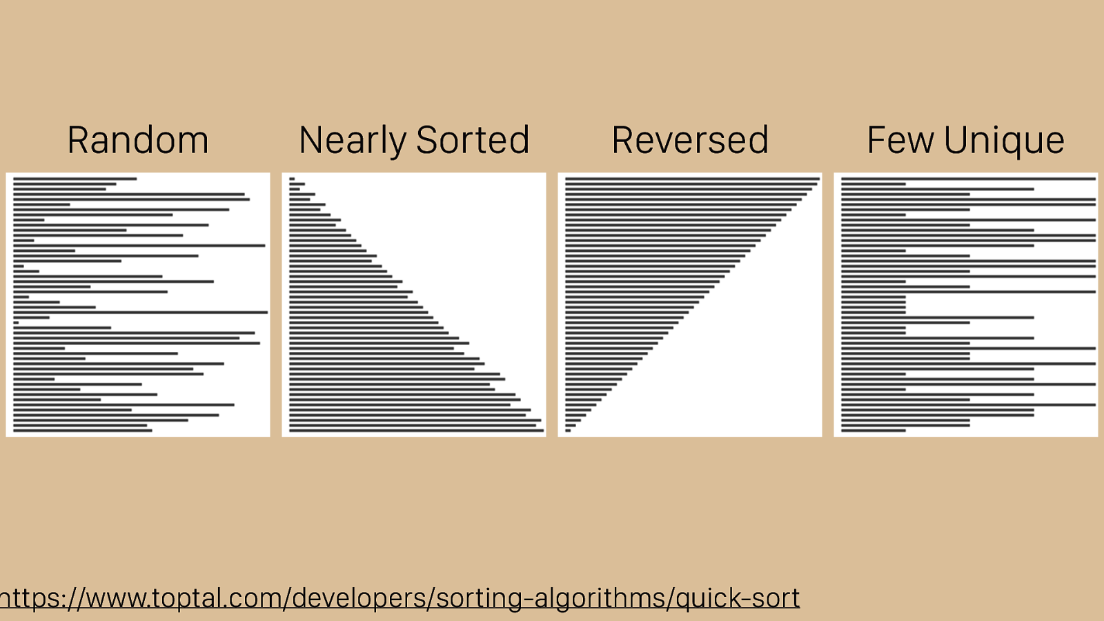
https://www.toptal.com/developers/sorting-algorithms/bubble-sort Random Nearly Sorted Reversed Few Unique It’s useful to see a visualization of how these algorithms work in different cases. Toptal has this great set of visualizations that show bubble sort operating over di ff erent types of inputs. These can help you build an intuition about how bubble sort will work in various cases. The red arrow indicates our “subject” which we used the sorting hat for, dark bars are sorted, and light bars are yet to be sorted. We have random, nearly sorted, reversed, and few unique sets of input data.

https://www.toptal.com/developers/sorting-algorithms/bubble-sort Random Nearly Sorted Reversed Few Unique It’s useful to see a visualization of how these algorithms work in different cases. Toptal has this great set of visualizations that show bubble sort operating over di ff erent types of inputs. These can help you build an intuition about how bubble sort will work in various cases. The red arrow indicates our “subject” which we used the sorting hat for, dark bars are sorted, and light bars are yet to be sorted. We have random, nearly sorted, reversed, and few unique sets of input data.

Insertion Sort Insertion sort is another simple algorithm. It’s very e ffi cient at sorting almost sorted or very small sets. Insertion sort is so called because it inserts the subject element into the subset of previously sorted elements in the correct order by comparing until it is greater than one of the previous elements and then inserting after that.

!"#"$"%"&"'"(")"*"+", So the algorithm: For each element, consider all elements to its left. Continue until you reach one that is smaller than the element or you run out of elements to check. If you found anything smaller, move the element just after that place and shift the larger elements to the right. Let’s take a look.

! "#"$"%"&"'"(")"*"+", We start with the first and compare it to everything to its left. This step is pretty easy, there’s nothing bigger to the left (since there’s nothing to the left), so we’re done.

!"

"$"%"&"'"(")"*"+", No we consider the next element.

! "

"$"%"&"'"(")"*"+", The red element we’re comparing is not bigger than the green subject. We don’t want to move anything here, as this subset is already sorted.

!"#" $ "%"&"'"(")"*"+", On to the next green subject.

!"

" $ "%"&"'"(")"*"+", We’ll compare each of these

! "#" $ "%"&"'"(")"*"+", and see that they’re both smaller.

!"#"$" % "&"'"(")"*"+", Next!

!"#" $ " % "&"'"(")"*"+", This one’s bigger

!"

"$" % "&"'"(")"*"+", But so is this

! "#"$" % "&"'"(")"*"+", and this

% "!"#"$"&"'"(")"*"+", So we shift the green subject before all of them. Now the first four elements are in order.

We’ll repeat this until the whole set is sorted. Let’s speed through that.

%"!"#"$" & "'"(")"*"+",

%"!"#" $ " & "'"(")"*"+",

%"!"

"$" & "'"(")"*"+",

%" ! "#"$" & "'"(")"*"+",

% "!"#"$" & "'"(")"*"+",

%" & "!"#"$"'"(")"*"+",

%"&"!"#"$" ' "(")"*"+",

%"&"!"#" $ " ' "(")"*"+",

%"&"!"

"$" ' "(")"*"+",

%"&" ! "#"$" ' "(")"*"+",

%" & "!"#"$" ' "(")"*"+",

% "&"!"#"$" ' "(")"*"+",

' "%"&"!"#"$"(")"*"+",

'"%"&"!"#"$" ( ")"*"+",

'"%"&"!"#" $ " ( ")"*"+",

'"%"&"!"

"$" ( ")"*"+",

'"%"&" ! "#"$" ( ")"*"+",

'"%" & "!"#"$" ( ")"*"+",

'" % "&"!"#"$" ( ")"*"+",

' "%"&"!"#"$" ( ")"*"+",

( "'"%"&"!"#"$")"*"+",

("'"%"&"!"#"$" ) "*"+",

("'"%"&"!"#" $ " ) "*"+",

("'"%"&"!"

"$" ) "*"+",

("'"%"&" ! "#"$" ) "*"+",

("'"%" & "!"#"$" ) "*"+",

("'"%"&" ) "!"#"$"*"+",

("'"%"&")"!"#"$" * "+",

("'"%"&")"!"#" $ " * "+",

("'"%"&")"!"

"$" * "+",

("'"%"&")" ! "#"$" * "+",

("'"%"&")"!" * "#"$"+",

("'"%"&")"!"*"#"$" + ",

("'"%"&")"!"*"#" $ " + ",

("'"%"&")"!"*"

"$" + ",

("'"%"&")"!" * "#"$" + ",

("'"%"&")" ! "*"#"$" + ",

("'"%"&" ) "!"*"#"$" + ",

("'"%" & ")"!"*"#"$" + ",

("'"%"&" + ")"!"*"#"$",

("'"%"&"+")"!"*"#"$" ,

("'"%"&"+")"!"*"#" $ " ,

("'"%"&"+")"!"*"

"$" ,

("'"%"&"+")"!" * "#"$" ,

("'"%"&"+")" ! "*"#"$" ,

("'"%"&"+" ) "!"*"#"$" ,

("'"%"&"+")" , "!"*"#"$

("'"%"&"+")","!"*"#"$ And now we have a sorted set. Insertion sort is a fun one because it’s one of the simplest sorting algorithms to write.

2 ) n O ( Like bubble sort, Insertion sort operates in quadratic time both for Big O (worst case) and in the average case.

⌦ ( n ) Its Big Omega, or best case performance, is also the same as Bubble sort, linear time. Because of the inherent “lossiness” of Big O notation, this ignores that insertion sort tends to operate more e ffi ciently than bubble sort, but it’s definitely not a fantastic way to sort a large set.

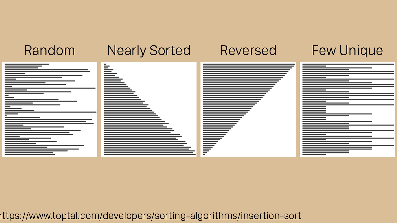
https://www.toptal.com/developers/sorting-algorithms/insertion-sort Random Nearly Sorted Reversed Few Unique Insertion sort does work very well on nearly sorted arrays. It’s already finished. Because of this, insertion sort is sometimes used as a “finishing step” for quicksort, which we’ll look at next. It shares the benefit bubble sort has of returning an already sorted set in linear time. You can see that it’s working much better on the reversed set and is generally faster, despite having the same complexity representations, than bubble sort.

https://www.toptal.com/developers/sorting-algorithms/insertion-sort Random Nearly Sorted Reversed Few Unique Insertion sort does work very well on nearly sorted arrays. It’s already finished. Because of this, insertion sort is sometimes used as a “finishing step” for quicksort, which we’ll look at next. It shares the benefit bubble sort has of returning an already sorted set in linear time. You can see that it’s working much better on the reversed set and is generally faster, despite having the same complexity representations, than bubble sort.

Quicksort Quicksort is often considered the “state of the art” in sorting algorithms. This is because the average case performance is very low for a comparison sorting algorithms. Quicksort’s algorithm is a bit different than bubble or insertion sort. Rather than moving the element we’re comparing against, which we call the pivot in quicksort, we move everything else around it to the left if it’s less than the pivot and the right if greater. Then we do the same thing for each set of things moved and continue until everything’s sorted.

2 ) n O ( Quicksort’s Big O is quadratic just like insertion or bubble sort. In the case of quicksort, it’s pretty rare to get this performance. To be n^2 operations, you’d need to always pick a pivot that was either the largest or smallest element, such that the remaining subsets to be quick sorted are of size 0 and n-1.

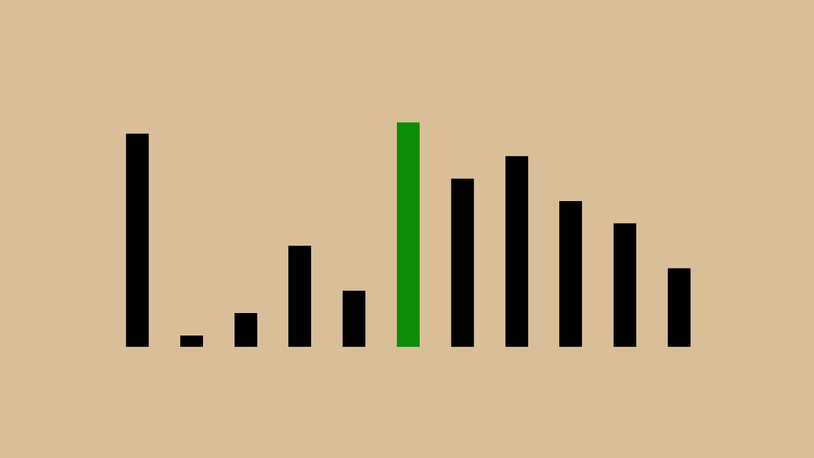
#"("'"+"%" $ "!"*",")"& We saw this in the very first operation in when the pivot we chose was the largest

#"("'"+"%"!"*",")"&" $ And the next subset was the whole set except the first pivot.

O ( n log n ) The magic of quick sort is that in the average case, its performance is linearithmic (the fancy word for n log n time). Average case here is not just intuition. There are several mathematical proofs that show this performance, but they’re over my head and out of scope for this talk.

⌦ ( n log n ) Linearithmic (or n log n) performance is also the best case for quicksort. So while quick sort isn’t always the fastest algorithm and can be just as slow as insertion or bubble sort given specific inputs, its average case is its best case, and the best case is pretty quick compared do others in this type of sorting algorithm. For general purposes (meaning integers, strings, whatever), this is the cream of the crop.

https://www.toptal.com/developers/sorting-algorithms/quick-sort Random Nearly Sorted Reversed Few Unique That said, it does have its weaknesses. While you can see that it does great with the reversed, nearly sorted, and random sets it has trouble with few unique set.

https://www.toptal.com/developers/sorting-algorithms/quick-sort Random Nearly Sorted Reversed Few Unique That said, it does have its weaknesses. While you can see that it does great with the reversed, nearly sorted, and random sets it has trouble with few unique set.

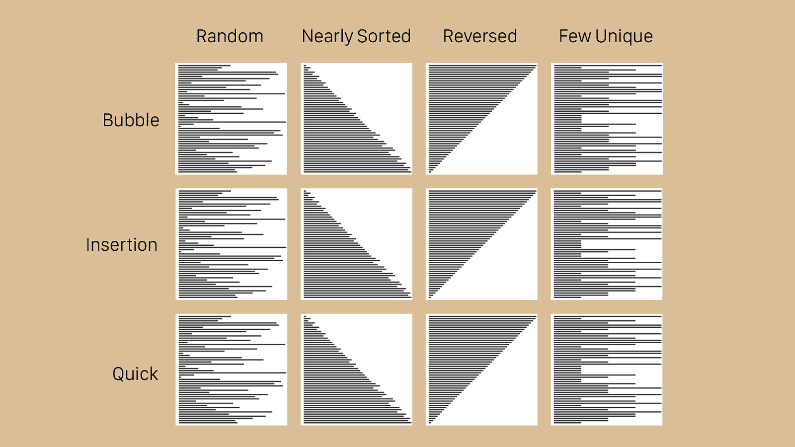
Bubble Random Nearly Sorted Reversed Few Unique Insertion Quick Here you can see the same visualizations we’ve looked at for each type of algorithm, all compared together. As the different algorithms work and finish, you can begin to see that some of them are better suited for specific tasks. The random set in the first column is a fair approximation of the average case, and you can see that quick sort works quickly there. It also makes short work of the reversed set, which trips up a lot of sorting algorithms. Insertion sort works very quickly for the nearly sorted set, and even bubble sort outperforms quick sort in this case. None of these algorithms work well with the few unique set. On the other hand, it’s di ffi cult to beat insertion sort or bubble sort for ease of writing the code. Perhaps most importantly however, quick sort provides very good average case results. This is why it is used in Ruby’s Array#sort implementation.

Bubble Random Nearly Sorted Reversed Few Unique Insertion Quick Here you can see the same visualizations we’ve looked at for each type of algorithm, all compared together. As the different algorithms work and finish, you can begin to see that some of them are better suited for specific tasks. The random set in the first column is a fair approximation of the average case, and you can see that quick sort works quickly there. It also makes short work of the reversed set, which trips up a lot of sorting algorithms. Insertion sort works very quickly for the nearly sorted set, and even bubble sort outperforms quick sort in this case. None of these algorithms work well with the few unique set. On the other hand, it’s di ffi cult to beat insertion sort or bubble sort for ease of writing the code. Perhaps most importantly however, quick sort provides very good average case results. This is why it is used in Ruby’s Array#sort implementation.

Gracias.

Bibliography • Pollice, G., Selkow, S., Heineman, G.T. (2008). Algorithms in a Nutshell . O’Reilly Media, Inc. • Bhargava, A. (2016). Grokking Algorithms . Manning Publications. • du Sautoy, M. (Presenter), Overton, P. (Producer). (2015, September 24). The Secret Rules of Modern Living: Algorithms

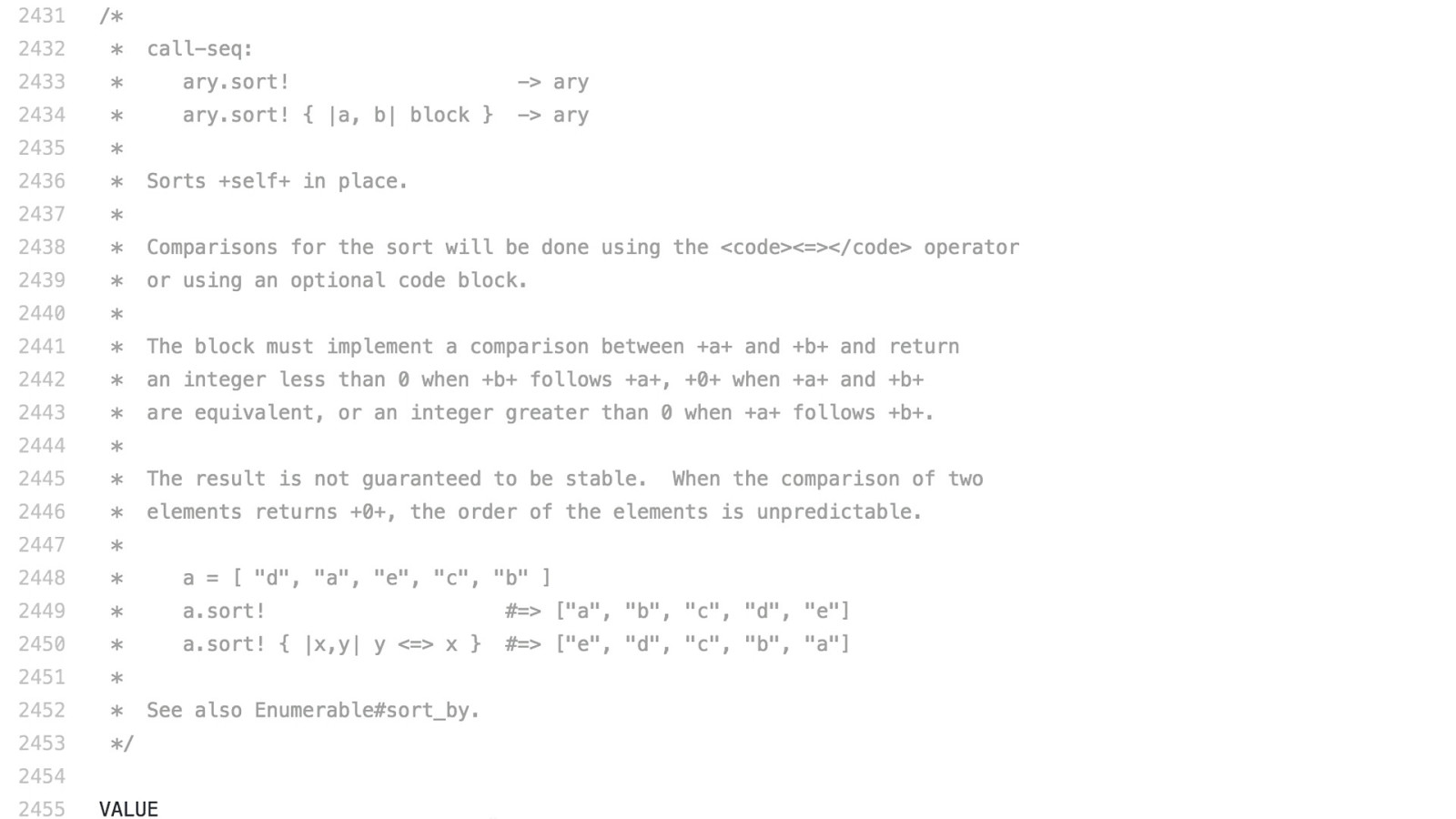
[Television broadcast]. London, UK: BBC Four. • Yukihiro, M. (1996). Array.sort!. Ruby [Software]. Retrieved 2017, March 27 from https://github.com/ruby/ruby/blob/ 47563655037ed453607de33b86fcc094878769ac/ array.c#L2431-L2513.

Images • Toptal. (2010). [Sorting Algorithms Animations]. Retrieved March 26, 2017, from https://www.toptal.com/developers/sorting-algorithms

• Cortesi, A. (2010). [sorting algorithm visualization]. Retrieved March 26, 2017, from http://sortvis.org/

• http://chocolate.wikia.com/wiki/Chocolate_Chip_Cookie

• https://www.babble.com/best-recipes/anatomy-of-a-chocolate-chip-cookie/

• http://thequotablekitchen.com/thick-chewy-chocolate-chip-cookies/

• http://www.beachwoodreporter.com/tv/what_i_watched_last_night_55.php

• http://asegrad.tufts.edu/academics/explore-graduate-programs/computer- science

Funography • https://www.youtube.com/watch?v=kPRA0W1kECg

• https://www.youtube.com/watch?v=gOKVwRIyWdg

• Big O and Big Omega graphics: https://texblog.org/ 2014/06/24/big-o-and-related-notations-in-latex/