How to Make Your Data Processing Faster - Parallel Processing and JIT in Data Science

How to Make Your Data Processing Faster - Parallel Processing and JIT in Data Science Presented by: Ong Chin Hwee (@ongchinhwee) 31 August 2019 Women Who Code Connect Asia, Singapore

About me ● Current role: Data Engineer at ST Engineering ● Background in aerospace engineering and computational modelling ● Experience working on aerospace-related projects in collaboration with academia and industry partners ● Find me if you would like to chat about Industry 4.0 and flight + travel!

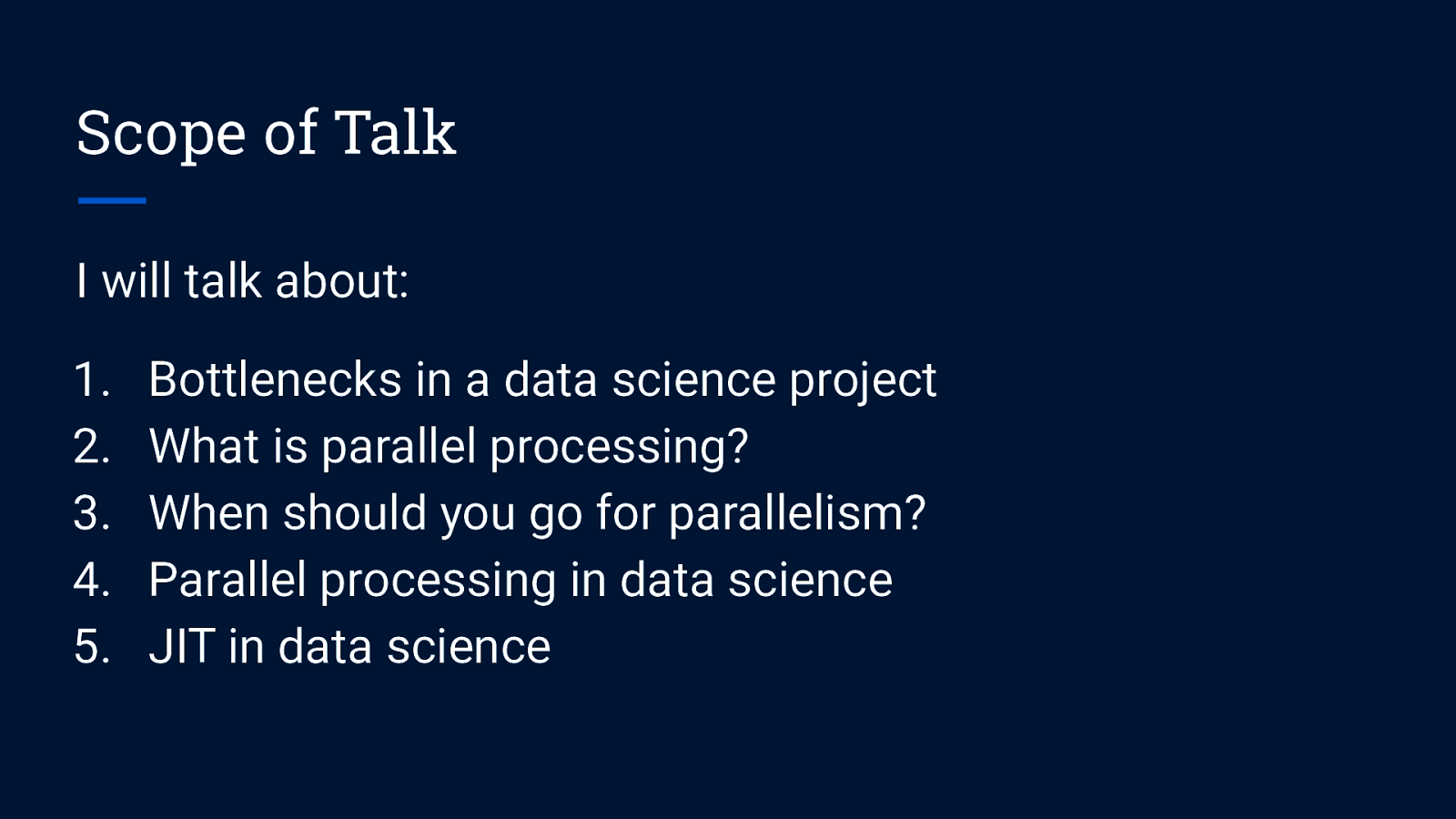
Scope of Talk I will talk about: 1. 2. 3. 4. 5. Bottlenecks in a data science project What is parallel processing? When should you go for parallelism? Parallel processing in data science JIT in data science

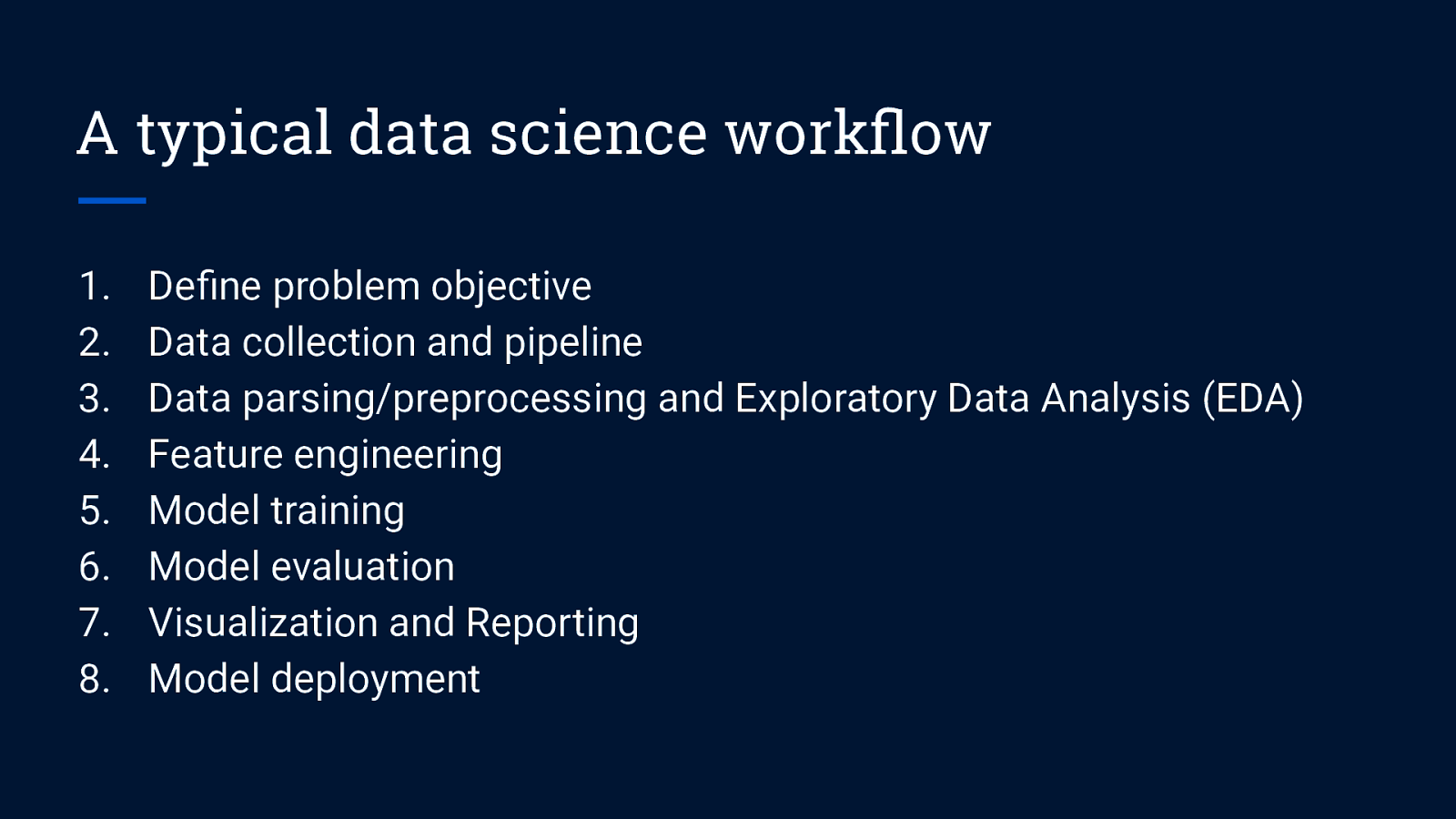
A typical data science workflow 1. 2. 3. 4. 5. 6. 7. 8. Define problem objective Data collection and pipeline Data parsing/preprocessing and Exploratory Data Analysis (EDA) Feature engineering Model training Model evaluation Visualization and Reporting Model deployment

What do you think are some of the bottlenecks in a data science project?

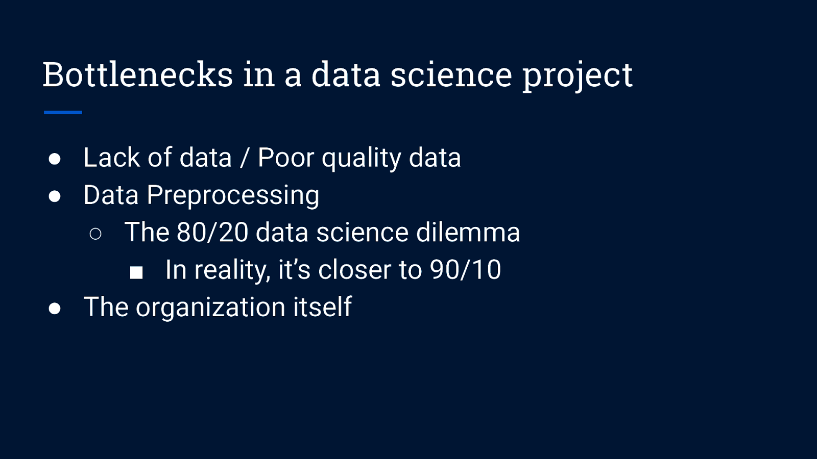
Bottlenecks in a data science project ● Lack of data / Poor quality data ● Data Preprocessing ○ The 80/20 data science dilemma ■ In reality, it’s closer to 90/10 ● The organization itself

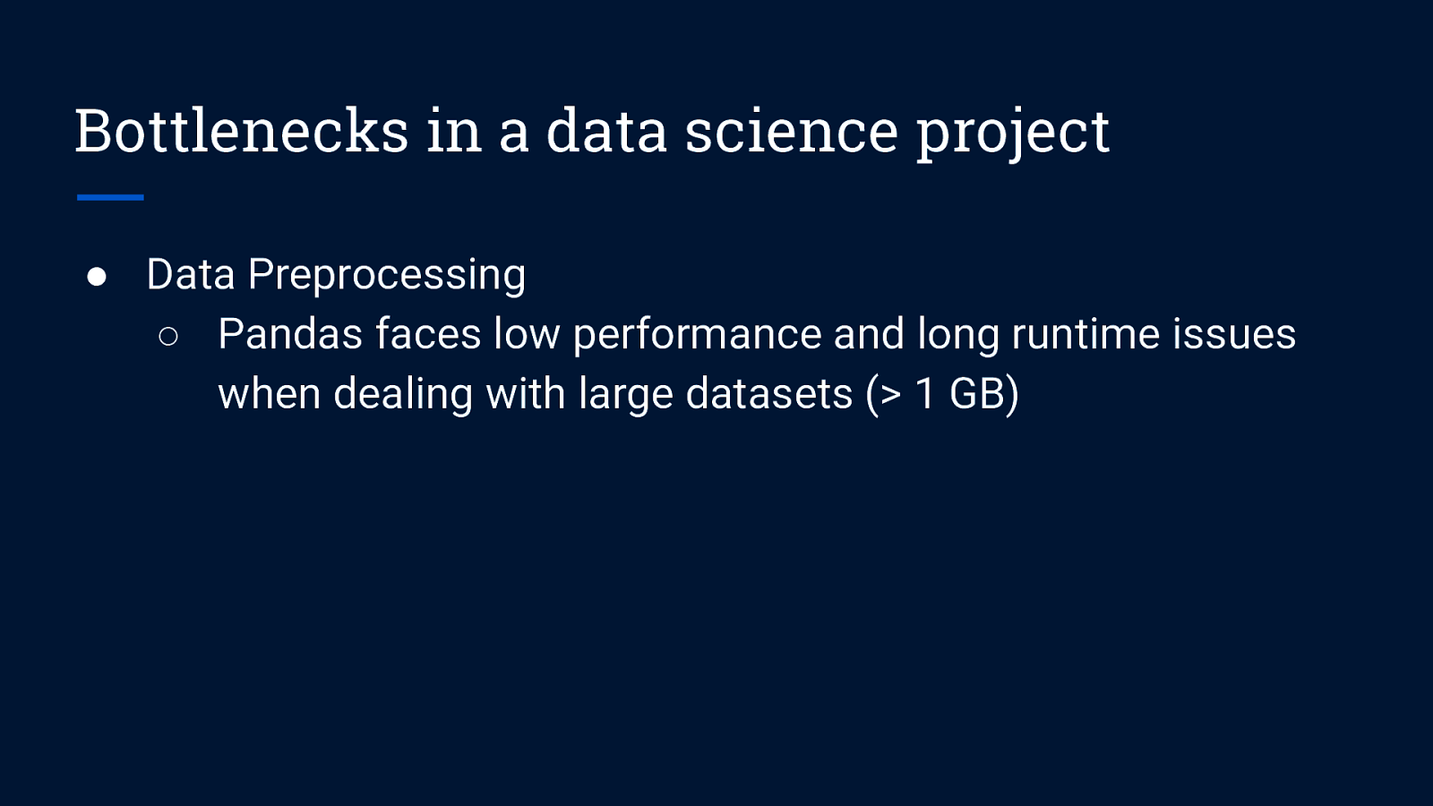
Bottlenecks in a data science project ● Data Preprocessing ○ Pandas faces low performance and long runtime issues when dealing with large datasets (> 1 GB)

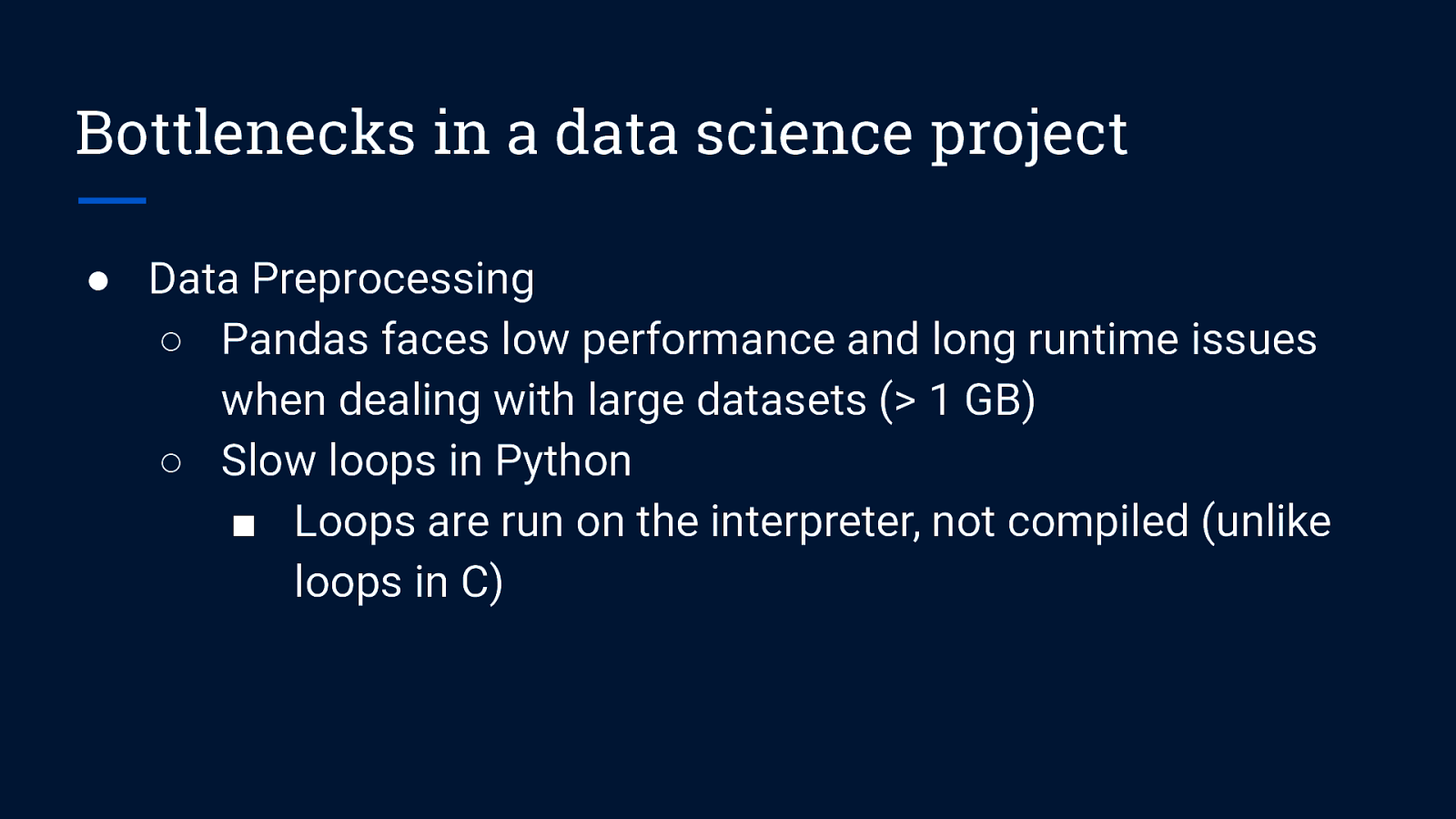
Bottlenecks in a data science project ● Data Preprocessing ○ Pandas faces low performance and long runtime issues when dealing with large datasets (> 1 GB) ○ Slow loops in Python ■ Loops are run on the interpreter, not compiled (unlike loops in C)

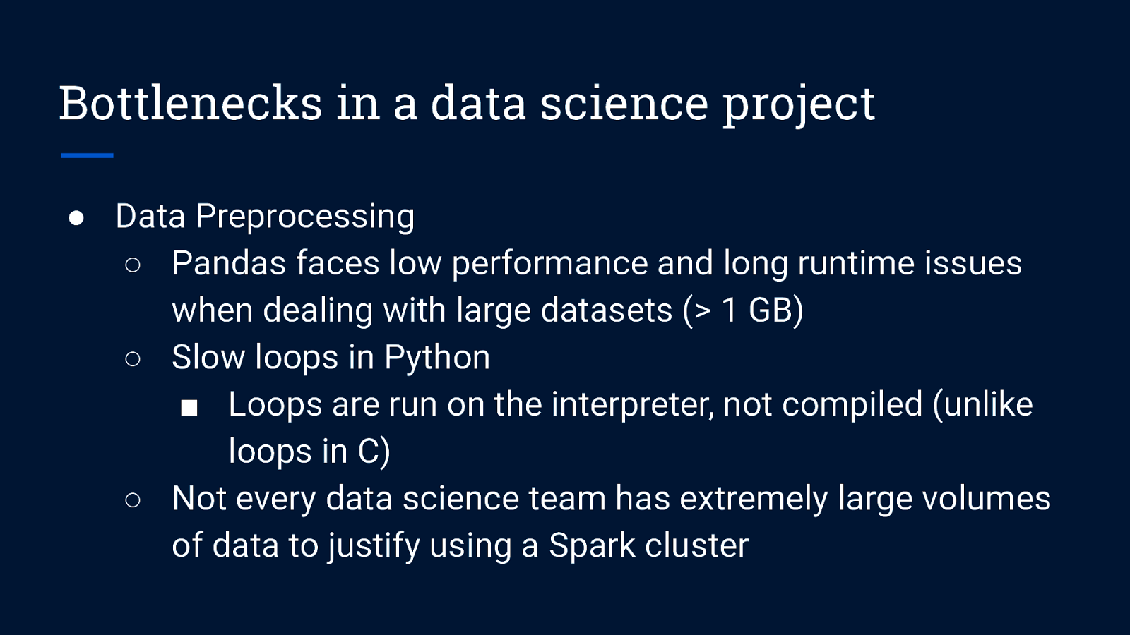
Bottlenecks in a data science project ● Data Preprocessing ○ Pandas faces low performance and long runtime issues when dealing with large datasets (> 1 GB) ○ Slow loops in Python ■ Loops are run on the interpreter, not compiled (unlike loops in C) ○ Not every data science team has extremely large volumes of data to justify using a Spark cluster

What is parallel processing?

Let’s imagine I own a bakery cafe.

Task 1: Toast 100 slices of bread Assumptions: 1. I’m using single-slice toasters. (Yes, they actually exist.) 2. Each slice of toast takes 2 minutes to make. 3. No overhead time. Image taken from: https://www.mitsubishielectric.co.jp/home/breadoven/product/to-st1-t/feature/index.html

Sequential Processing = 25 bread slices

Sequential Processing = 25 bread slices Processor/Worker: Toaster

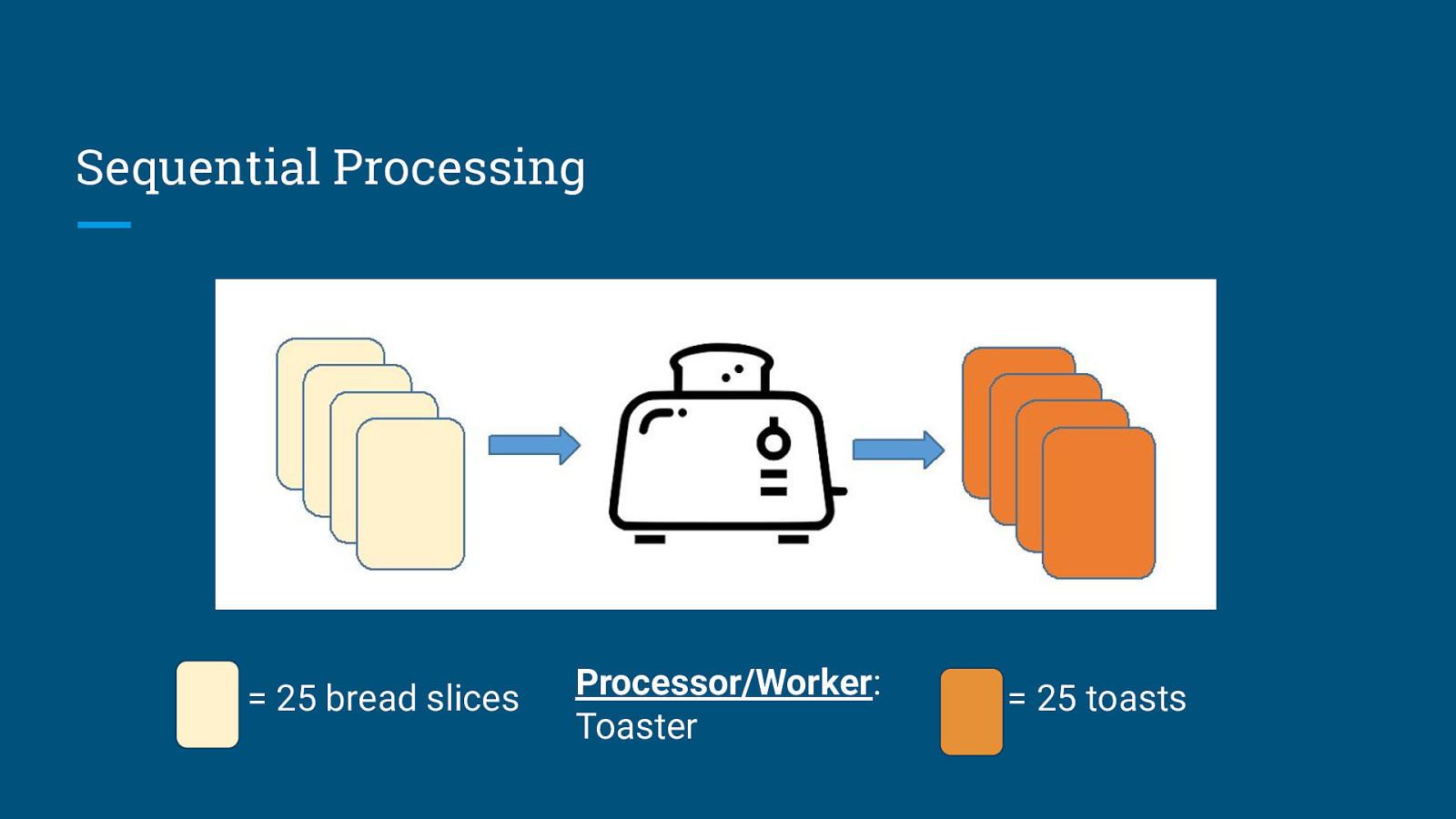
Sequential Processing = 25 bread slices Processor/Worker: Toaster = 25 toasts

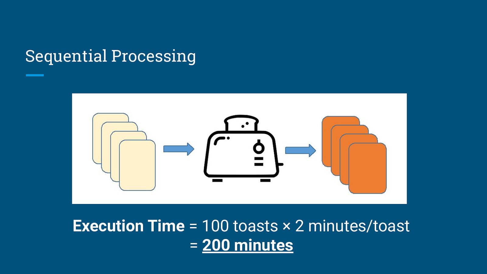
Sequential Processing Execution Time = 100 toasts × 2 minutes/toast = 200 minutes

Parallel Processing = 25 bread slices

Parallel Processing

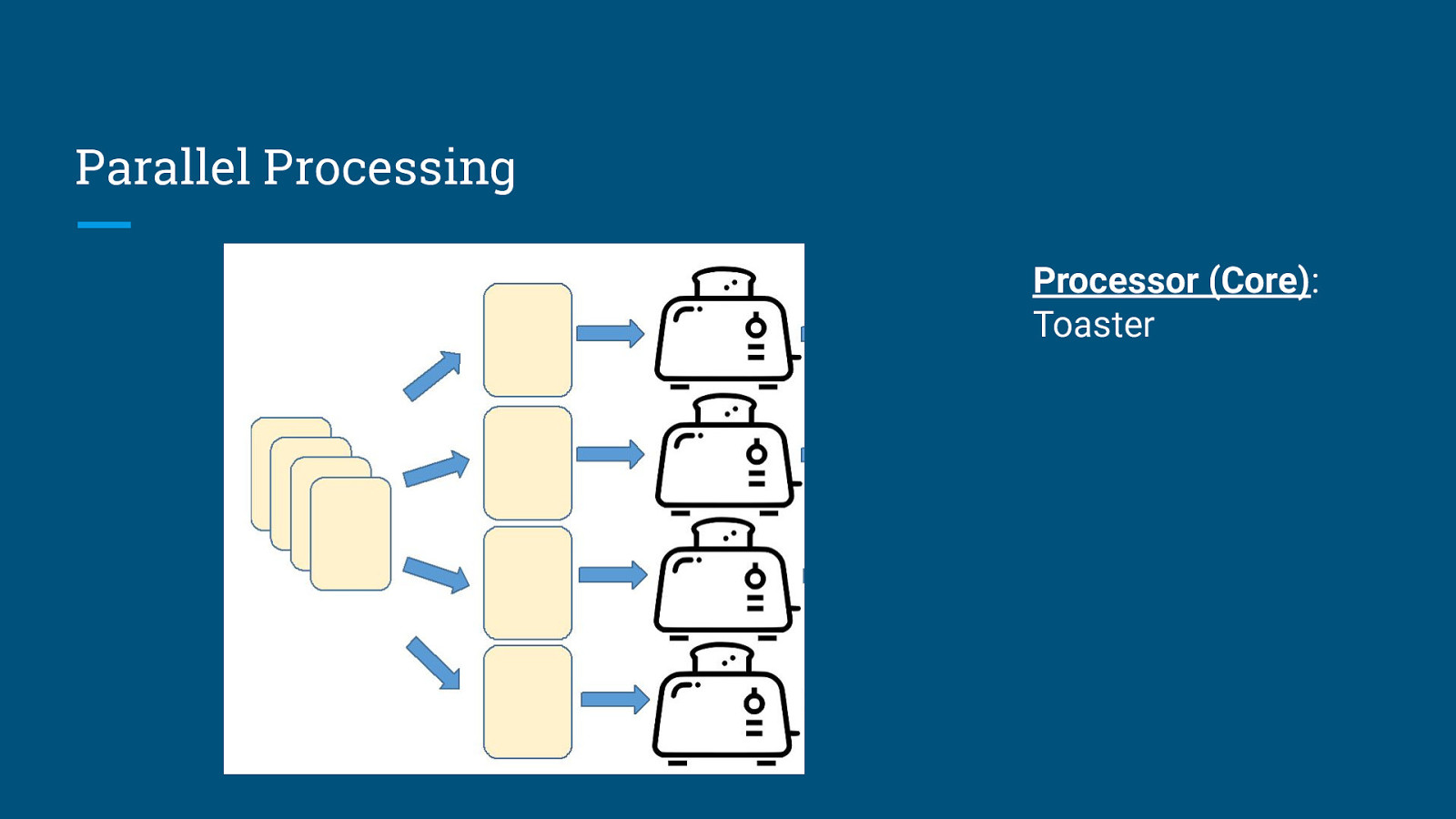
Parallel Processing Processor (Core): Toaster

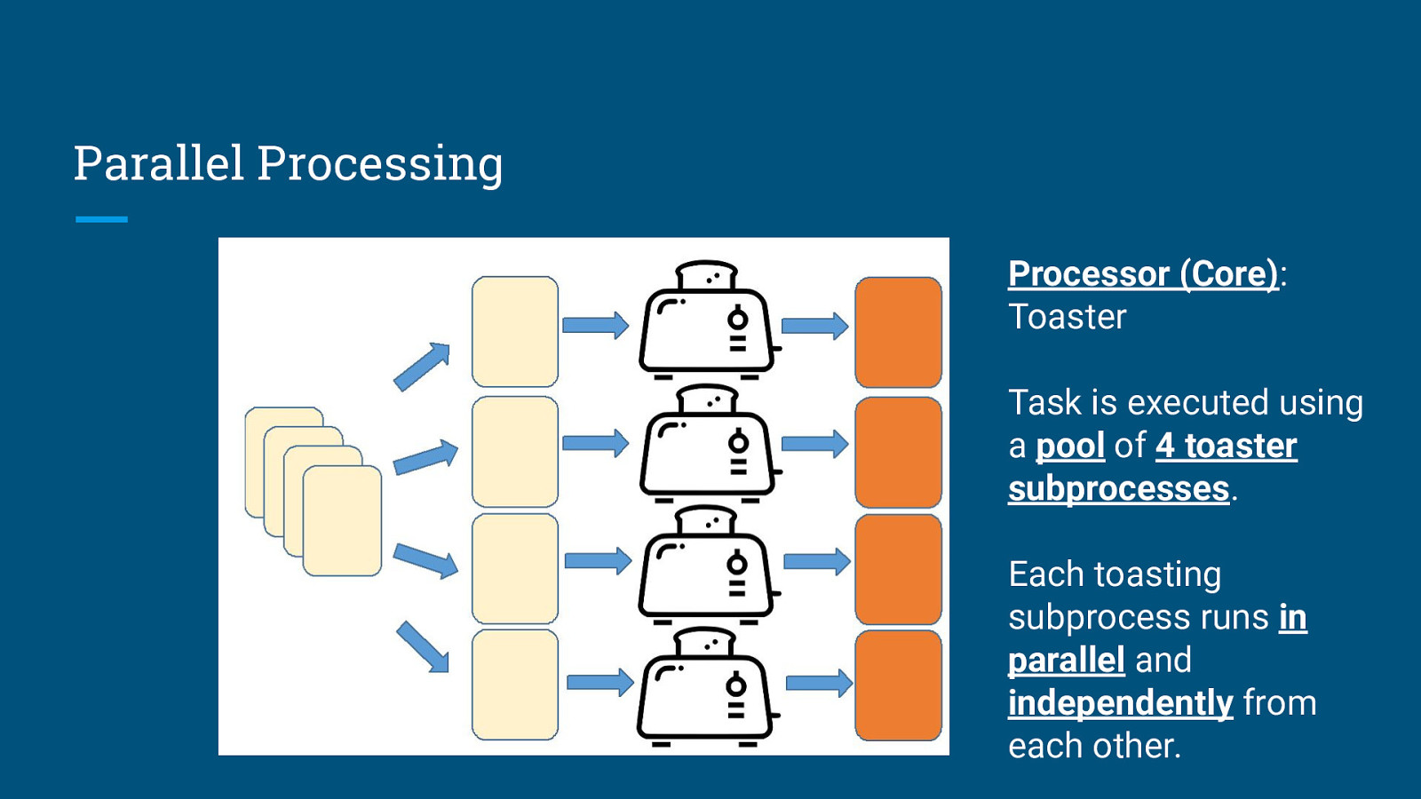
Parallel Processing Processor (Core): Toaster Task is executed using a pool of 4 toaster subprocesses. Each toasting subprocess runs in parallel and independently from each other.

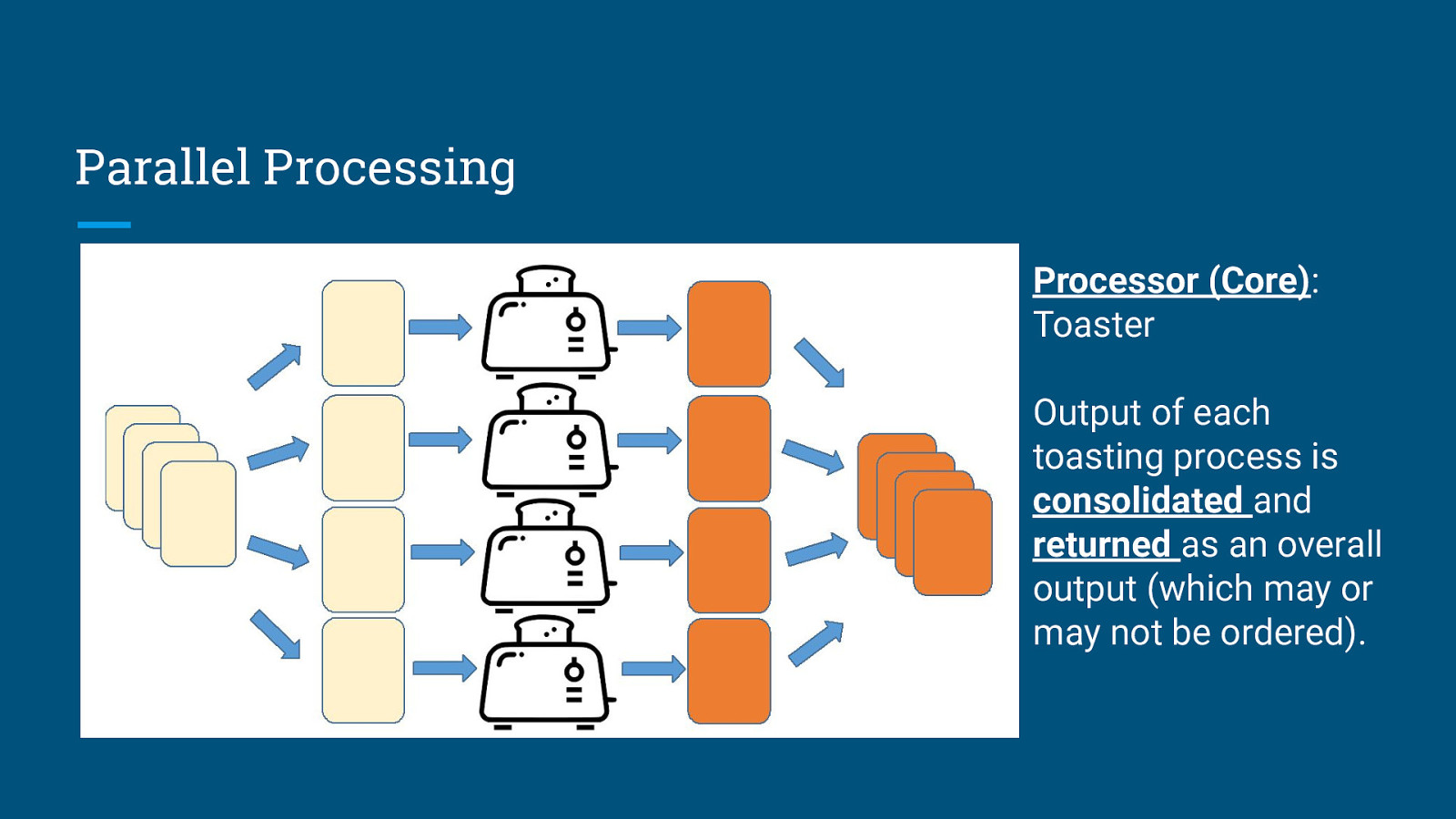
Parallel Processing Processor (Core): Toaster Output of each toasting process is consolidated and returned as an overall output (which may or may not be ordered).

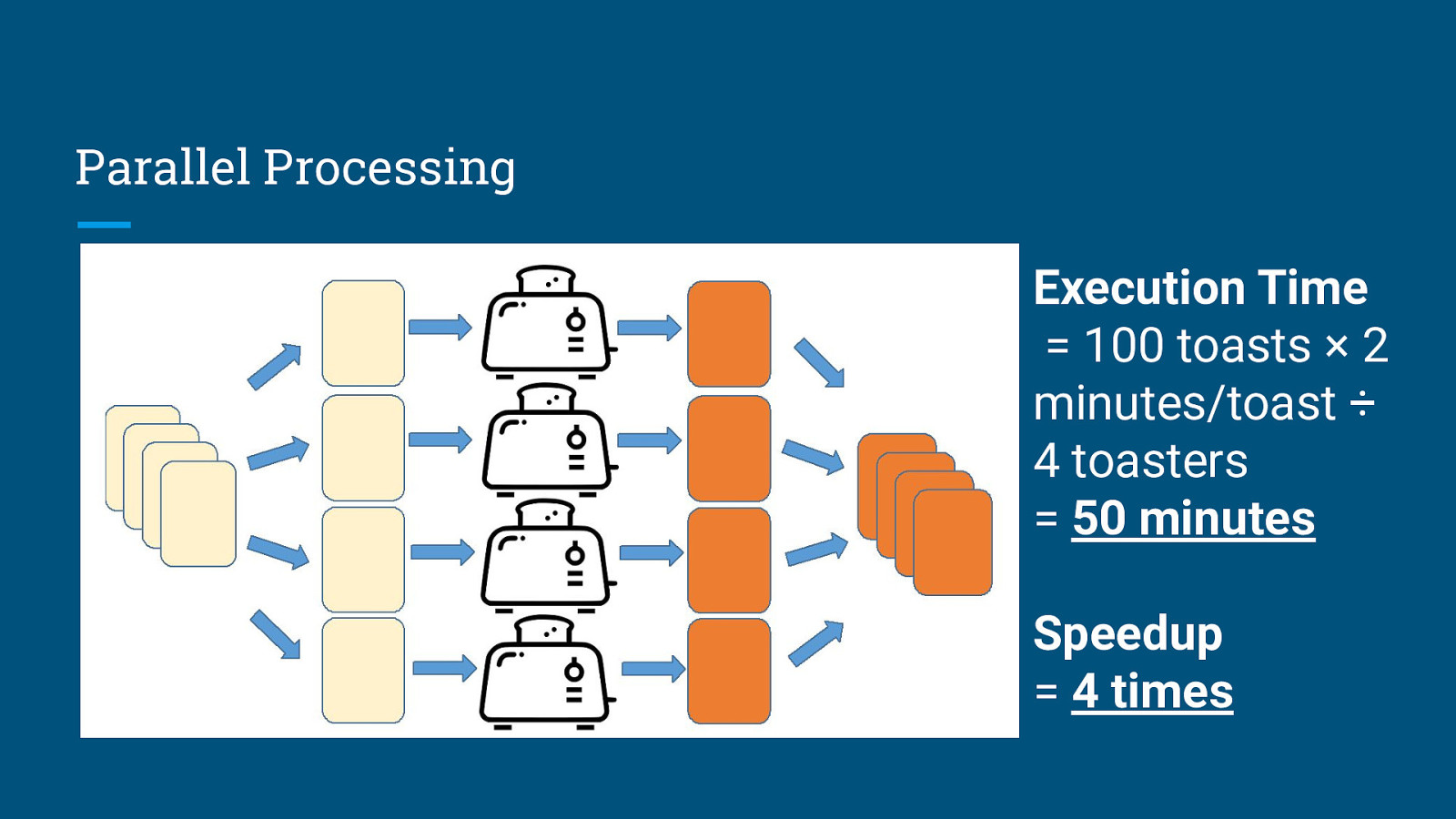
Parallel Processing Execution Time = 100 toasts × 2 minutes/toast ÷ 4 toasters = 50 minutes Speedup = 4 times

Synchronous vs Asynchronous Execution

What do you mean by “Asynchronous”?

Let’s get some ideas from the Kopi.JS folks. (since they do async programming more than the data folks)

me: One kopi pls (promise) Uncle: Ok, take this number and sit down, send to you when ready me: [sits down, surfs twitter] uncle: [walks over] order #23, here you go (async/await) uncle: Ok [makes kopi] me: [wait in place, surfs twitter] uncle: [kopi done] Here you go (Credits to: @sheldytox)

me: One kopi pls (promise) Uncle: Ok, take this number and sit down, send to you when ready me: [sits down, surfs twitter] uncle: [walks over] order #23, here you go (async/await) uncle: Ok [makes kopi] me: [wait in place, surfs twitter] uncle: [kopi done] Here you go (Credits to: @sheldytox) Another scenario, you wake up and order coffee via a delivery app. Do you wait by the phone for the coffee to arrive or do you go and do other things (while “awaiting” for the coffee to arrive)? (Credits to: @yingkh_tweets)

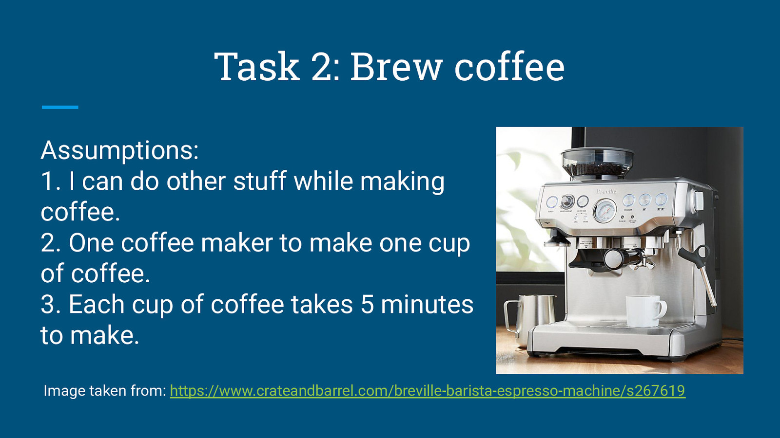
Task 2: Brew coffee Assumptions: 1. I can do other stuff while making coffee. 2. One coffee maker to make one cup of coffee. 3. Each cup of coffee takes 5 minutes to make. Image taken from: https://www.crateandbarrel.com/breville-barista-espresso-machine/s267619

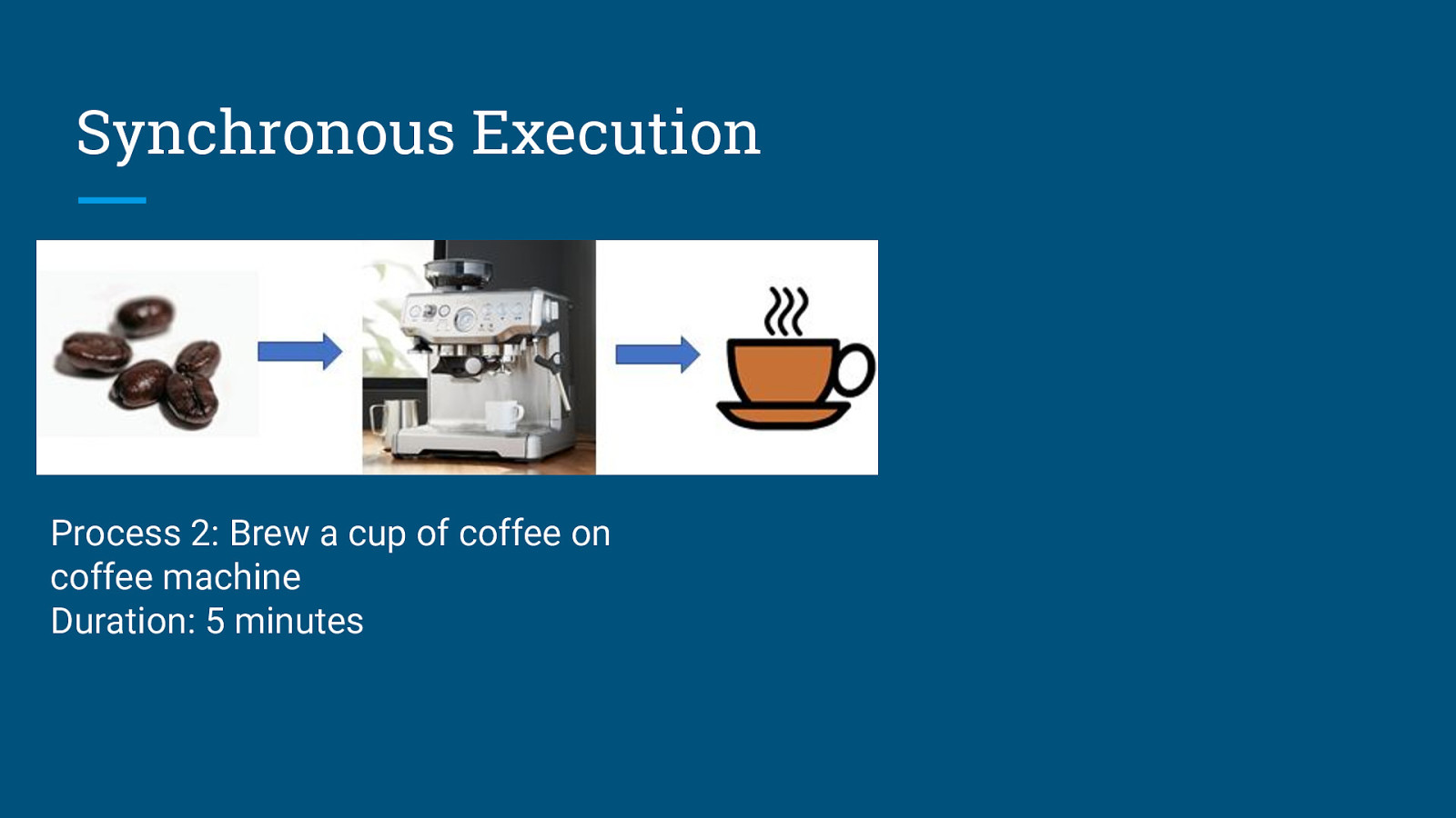
Synchronous Execution Process 2: Brew a cup of coffee on coffee machine Duration: 5 minutes

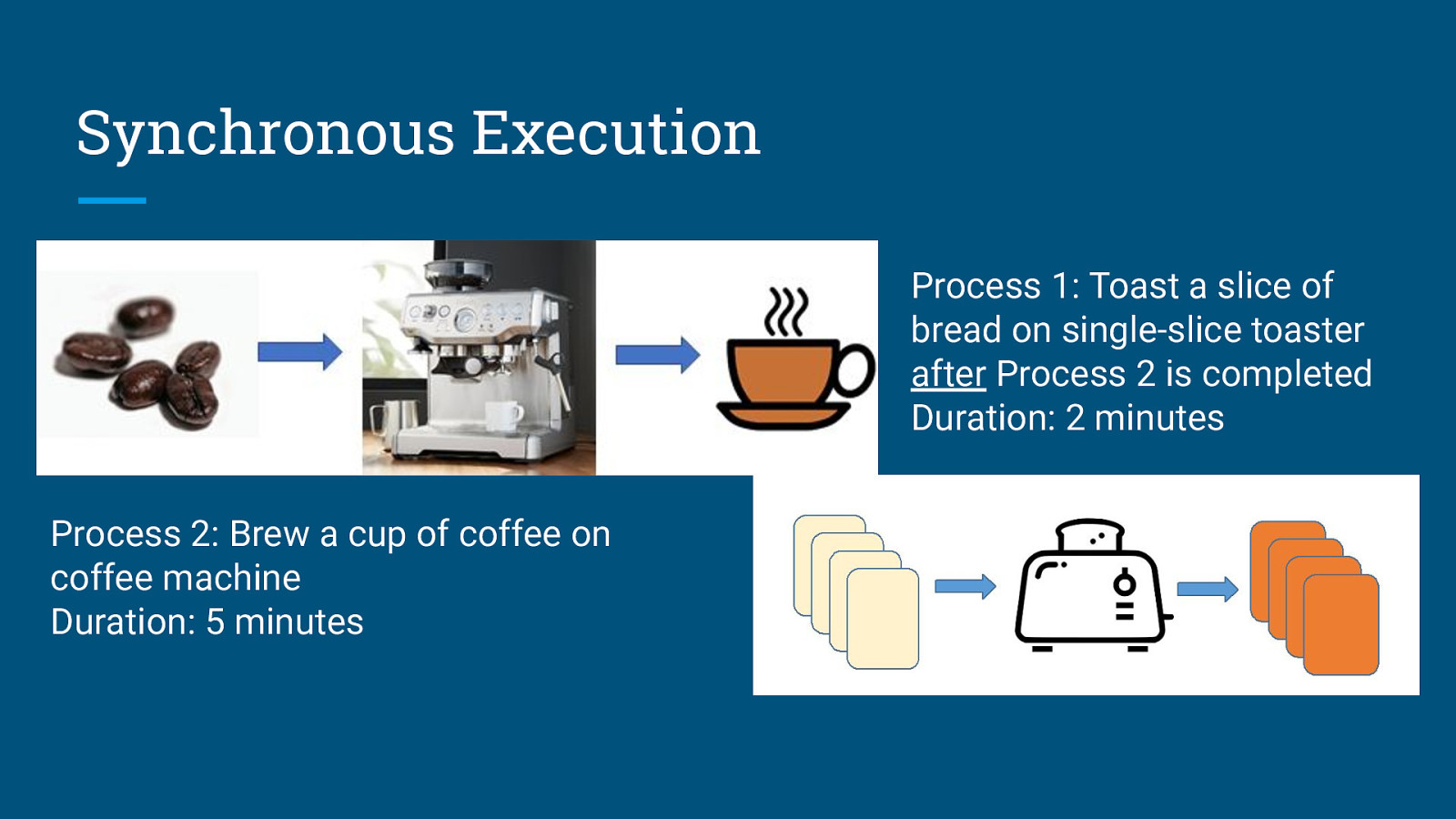
Synchronous Execution Process 1: Toast a slice of bread on single-slice toaster after Process 2 is completed Duration: 2 minutes Process 2: Brew a cup of coffee on coffee machine Duration: 5 minutes

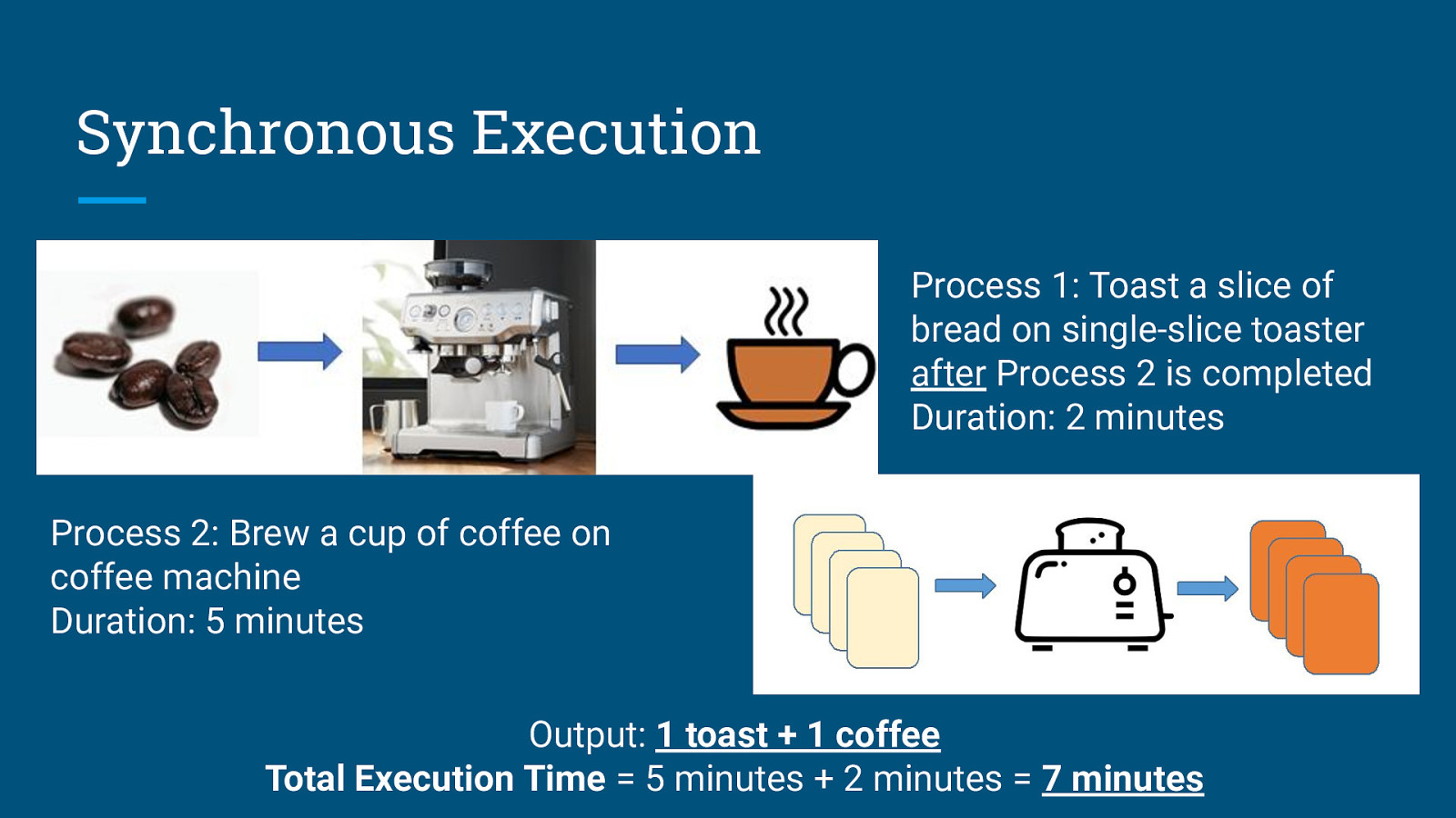
Synchronous Execution Process 1: Toast a slice of bread on single-slice toaster after Process 2 is completed Duration: 2 minutes Process 2: Brew a cup of coffee on coffee machine Duration: 5 minutes Output: 1 toast + 1 coffee Total Execution Time = 5 minutes + 2 minutes = 7 minutes

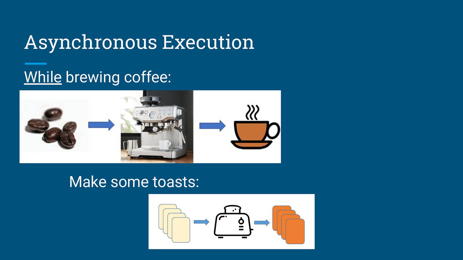
Asynchronous Execution While brewing coffee: Make some toasts:

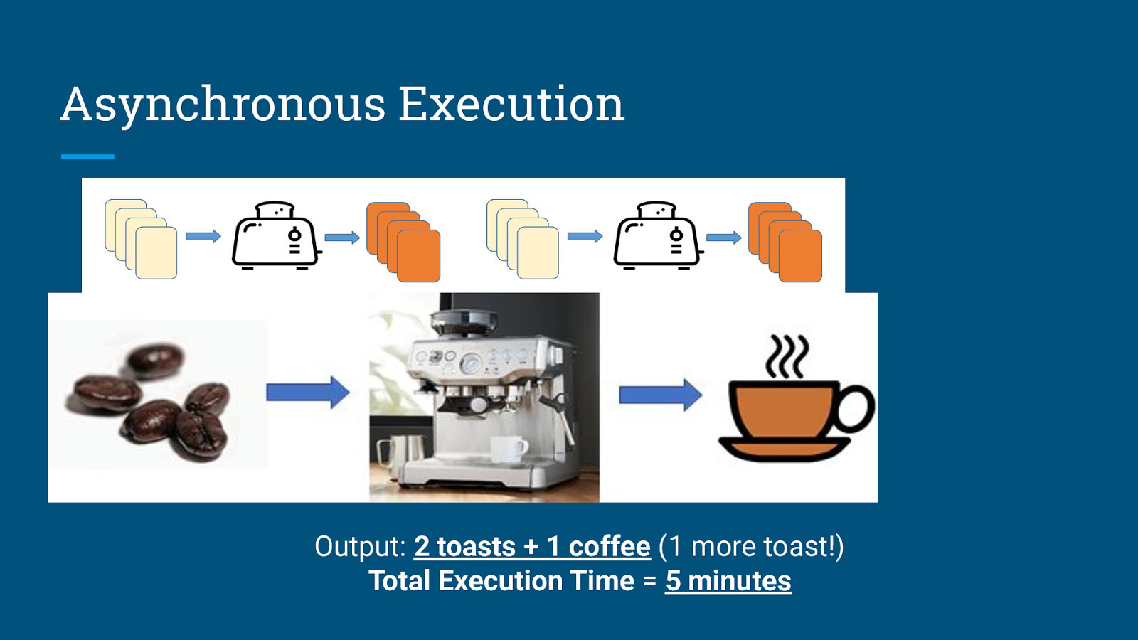
Asynchronous Execution Output: 2 toasts + 1 coffee (1 more toast!) Total Execution Time = 5 minutes

When is it a good idea to go for parallelism?

When is it a good idea to go for parallelism? (or, “Is it a good idea to simply buy a 256-core processor and parallelize all your codes?”)

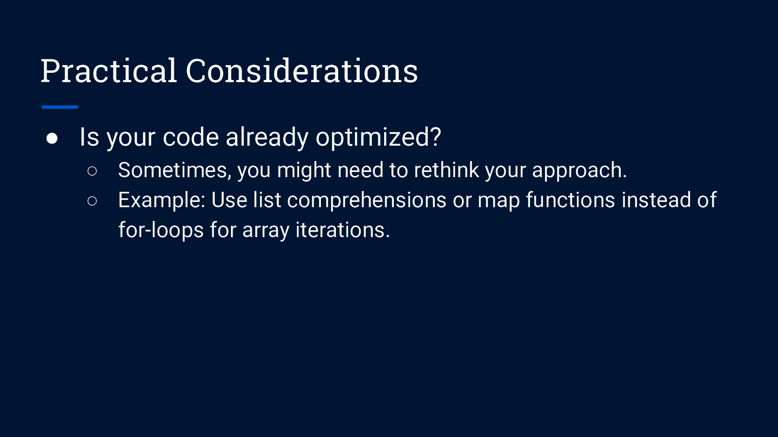
Practical Considerations ● Is your code already optimized? ○ Sometimes, you might need to rethink your approach. ○ Example: Use list comprehensions or map functions instead of for-loops for array iterations.

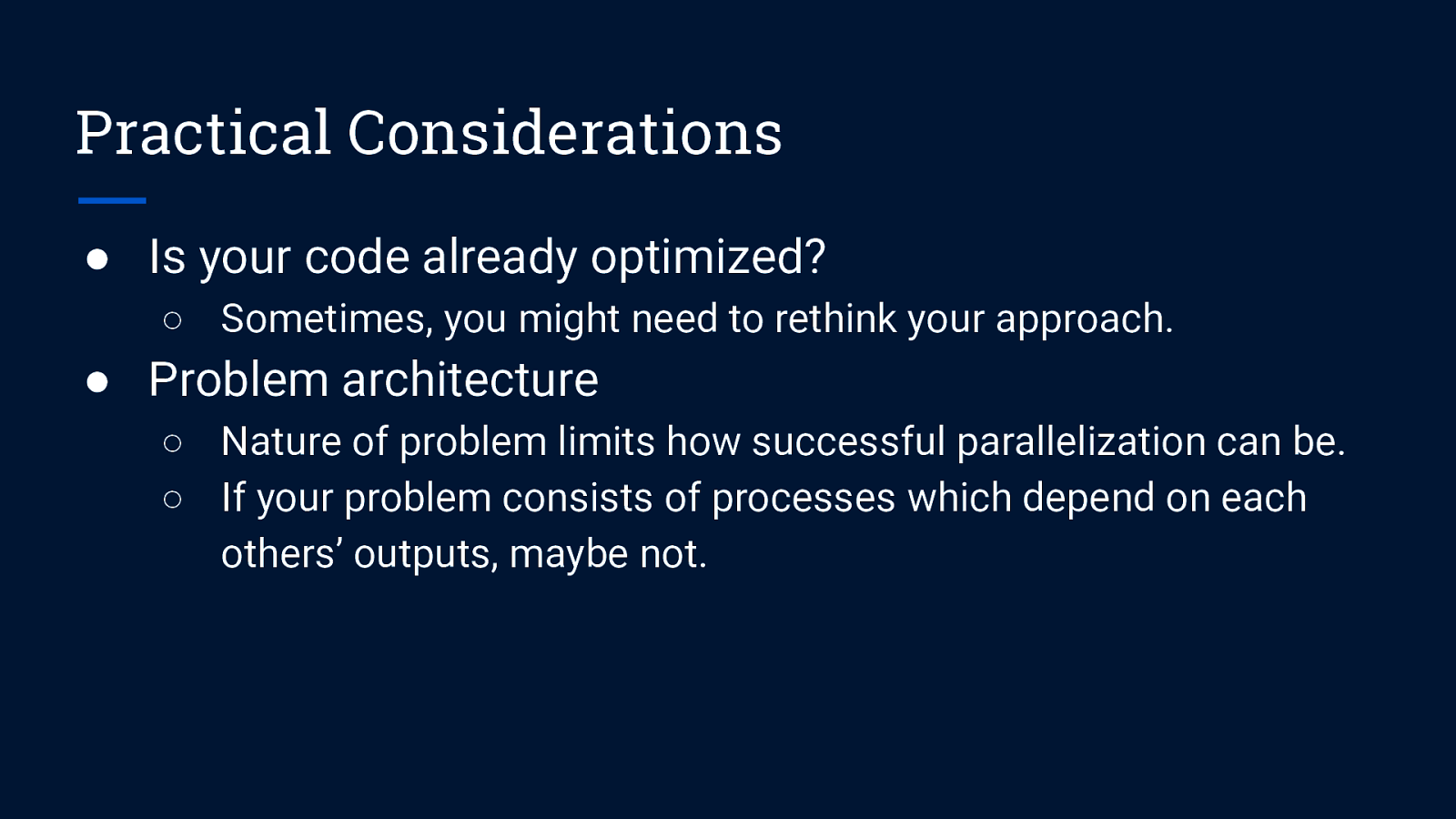
Practical Considerations ● Is your code already optimized? ○ Sometimes, you might need to rethink your approach. ● Problem architecture ○ Nature of problem limits how successful parallelization can be. ○ If your problem consists of processes which depend on each others’ outputs, maybe not.

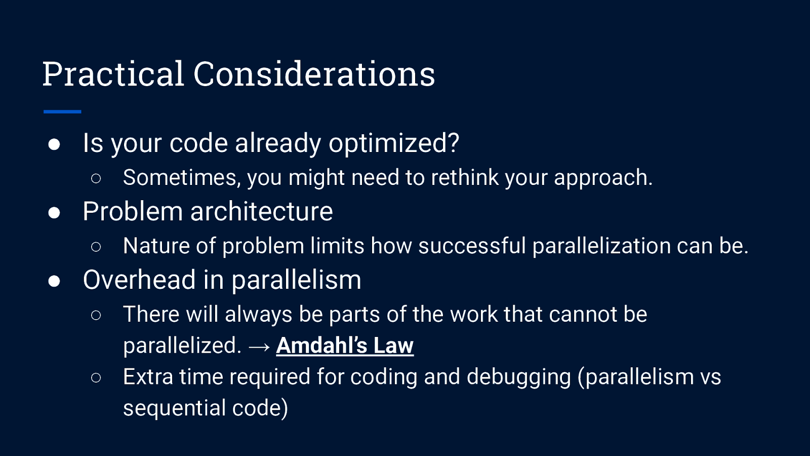
Practical Considerations ● Is your code already optimized? ○ Sometimes, you might need to rethink your approach. ● Problem architecture ○ Nature of problem limits how successful parallelization can be. ● Overhead in parallelism ○ There will always be parts of the work that cannot be parallelized. → Amdahl’s Law ○ Extra time required for coding and debugging (parallelism vs sequential code)

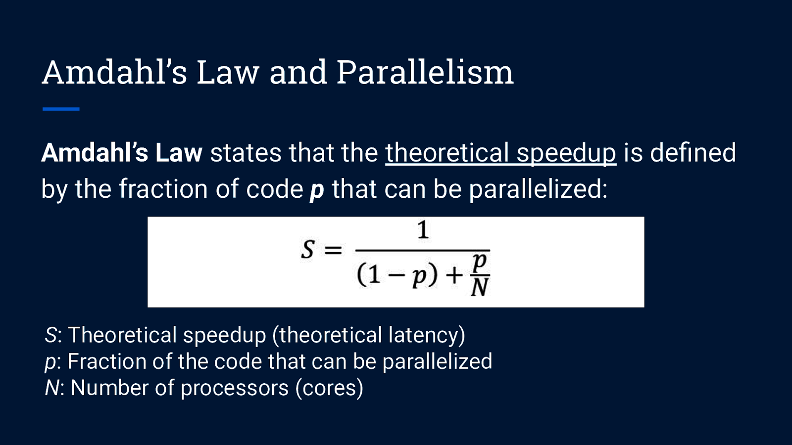
Amdahl’s Law and Parallelism Amdahl’s Law states that the theoretical speedup is defined by the fraction of code p that can be parallelized: S: Theoretical speedup (theoretical latency) p: Fraction of the code that can be parallelized N: Number of processors (cores)

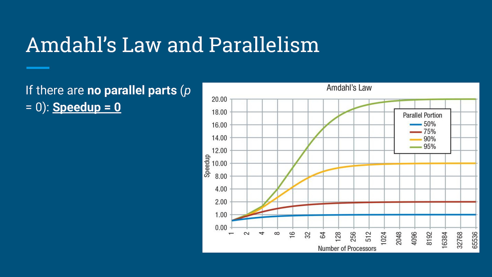
Amdahl’s Law and Parallelism If there are no parallel parts (p = 0): Speedup = 0

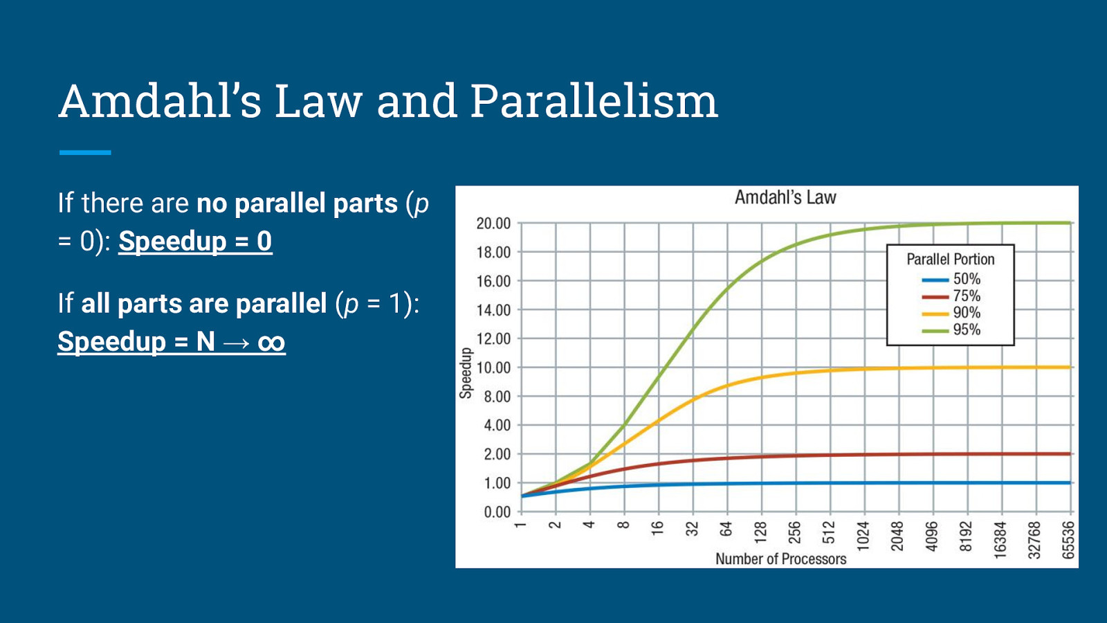
Amdahl’s Law and Parallelism If there are no parallel parts (p = 0): Speedup = 0 If all parts are parallel (p = 1): Speedup = N → ∞

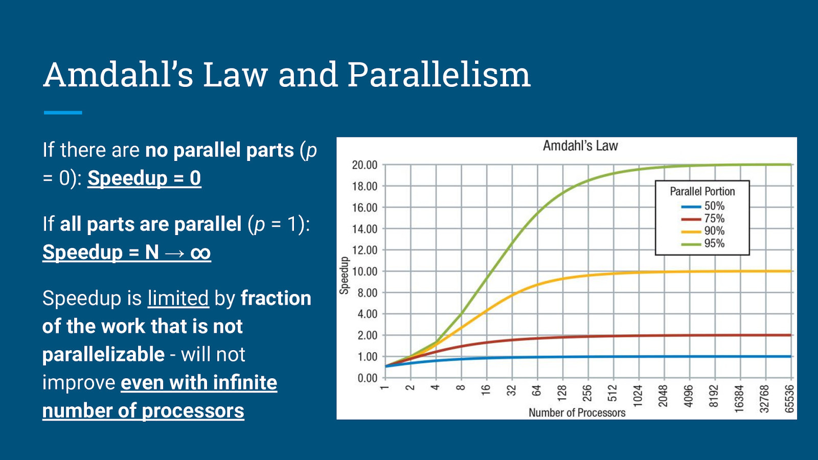
Amdahl’s Law and Parallelism If there are no parallel parts (p = 0): Speedup = 0 If all parts are parallel (p = 1): Speedup = N → ∞ Speedup is limited by fraction of the work that is not parallelizable - will not improve even with infinite number of processors

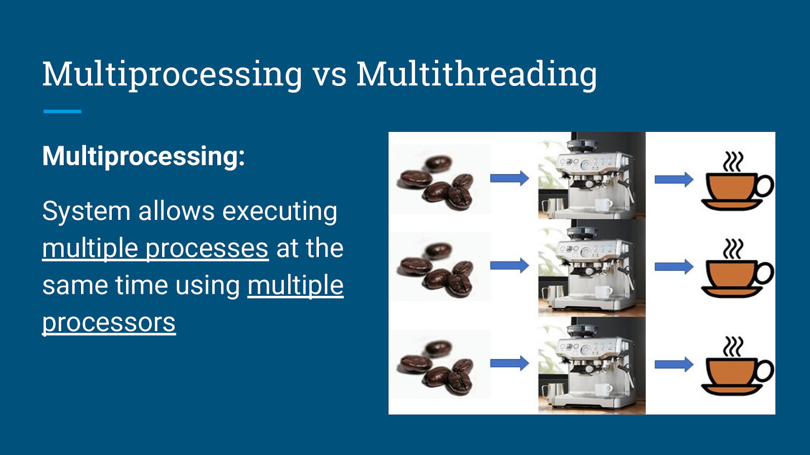
Multiprocessing vs Multithreading Multiprocessing: System allows executing multiple processes at the same time using multiple processors

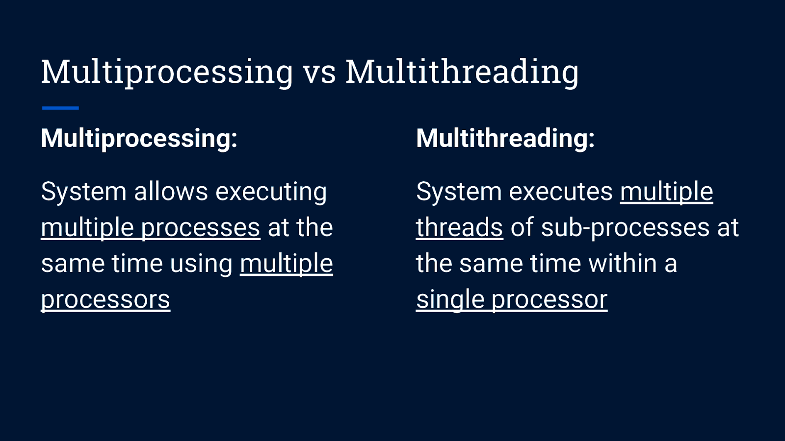
Multiprocessing vs Multithreading Multiprocessing: Multithreading: System allows executing multiple processes at the same time using multiple processors System executes multiple threads of sub-processes at the same time within a single processor

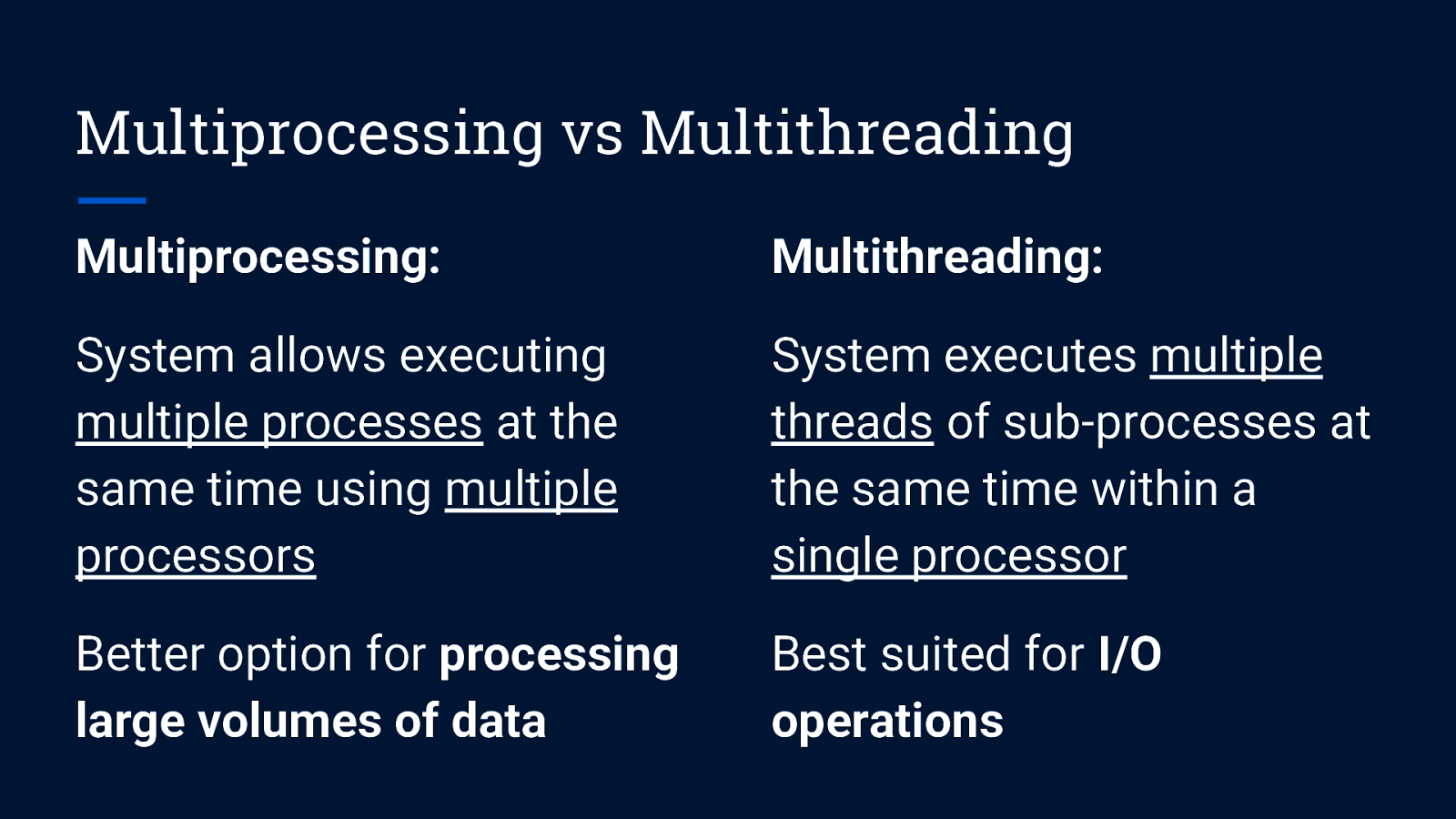
Multiprocessing vs Multithreading Multiprocessing: Multithreading: System allows executing multiple processes at the same time using multiple processors System executes multiple threads of sub-processes at the same time within a single processor Better option for processing large volumes of data Best suited for I/O operations

Parallel Processing in Data Science

Parallel Processing in Data Science Python is the most widely-used programming language in data science Distributed processing is one of the core concepts of Apache Spark Apache Spark is available in Python as PySpark

Parallel Processing in Data Science Data processing tends to be more compute-intensive → Switching between threads become increasingly inefficient → Global Interpreter Lock (GIL) in Python does not allow parallel thread execution

How to do Parallel Processing in Python?

Parallel Processing in Python concurrent.futures module ● High-level API for launching asynchronous parallel tasks ● Introduced in Python 3.2 as an abstraction layer over multiprocessing module ● Two modes of execution: ○ ThreadPoolExecutor() for multithreading ○ ProcessPoolExecutor() for multiprocessing

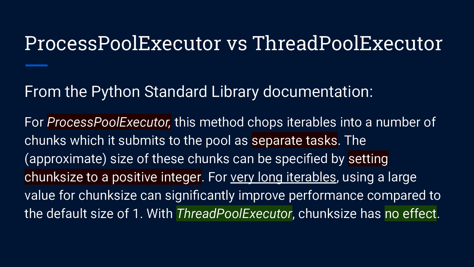
ProcessPoolExecutor vs ThreadPoolExecutor From the Python Standard Library documentation: For ProcessPoolExecutor, this method chops iterables into a number of chunks which it submits to the pool as separate tasks. The (approximate) size of these chunks can be specified by setting chunksize to a positive integer. For very long iterables, using a large value for chunksize can significantly improve performance compared to the default size of 1. With ThreadPoolExecutor, chunksize has no effect.

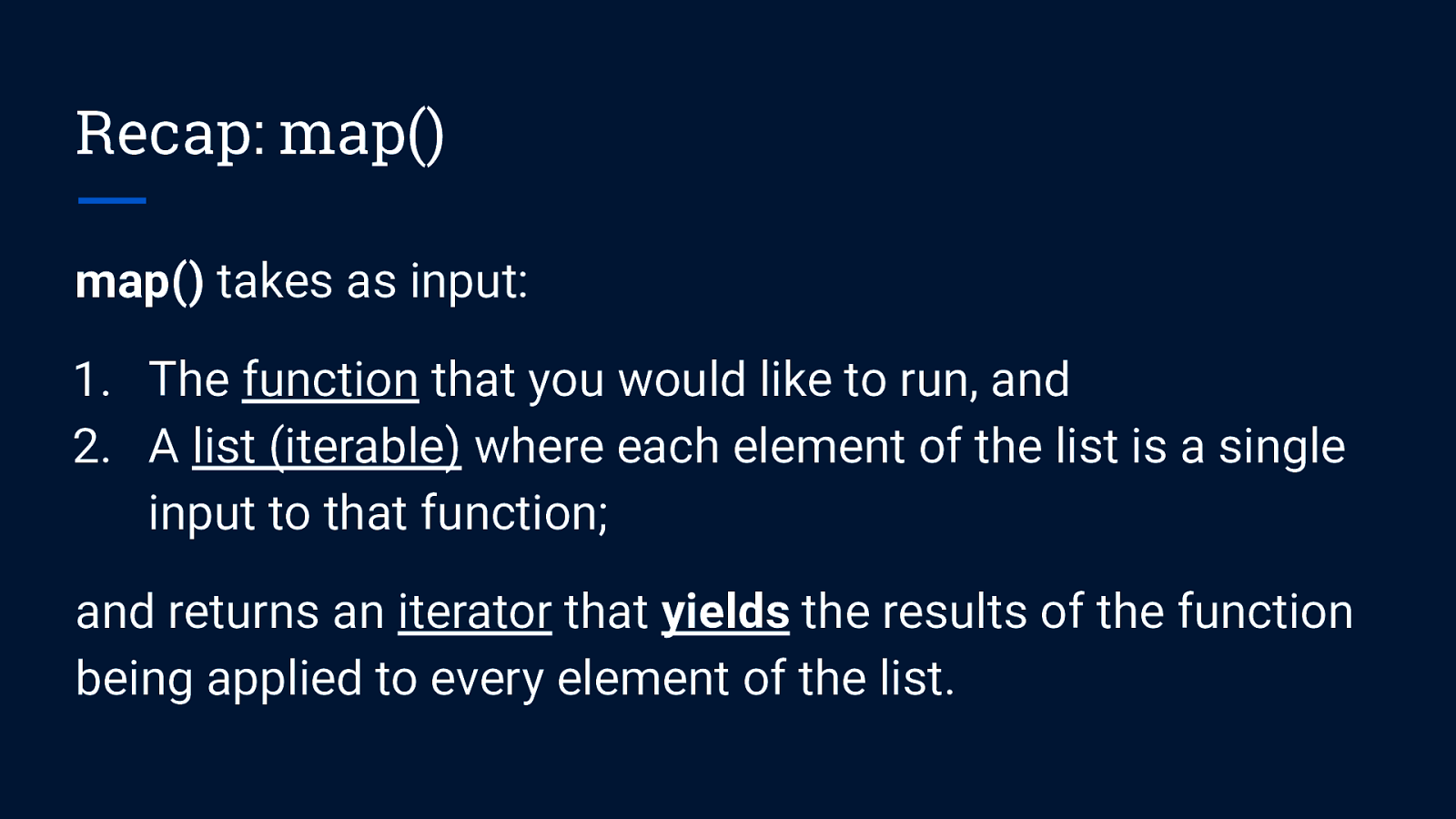
Recap: map() map() takes as input: 1. The function that you would like to run, and 2. A list (iterable) where each element of the list is a single input to that function; and returns an iterator that yields the results of the function being applied to every element of the list.

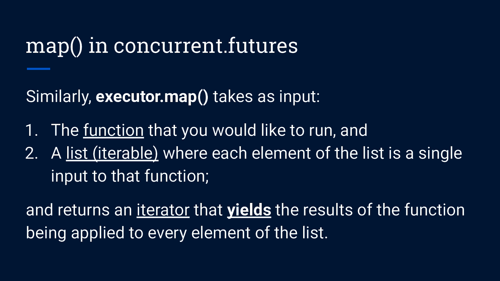
map() in concurrent.futures Similarly, executor.map() takes as input: 1. The function that you would like to run, and 2. A list (iterable) where each element of the list is a single input to that function; and returns an iterator that yields the results of the function being applied to every element of the list.

“Okay, I tried using parallel processing but my processing code in Python is still slow. What else can I do?”

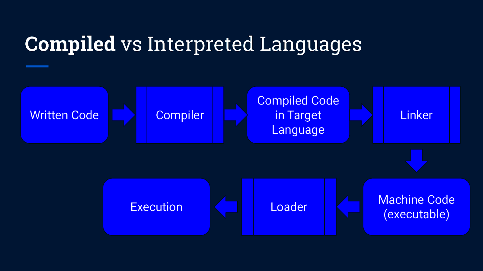
Compiled vs Interpreted Languages Written Code Compiler Execution Compiled Code in Target Language Loader Linker Machine Code (executable)

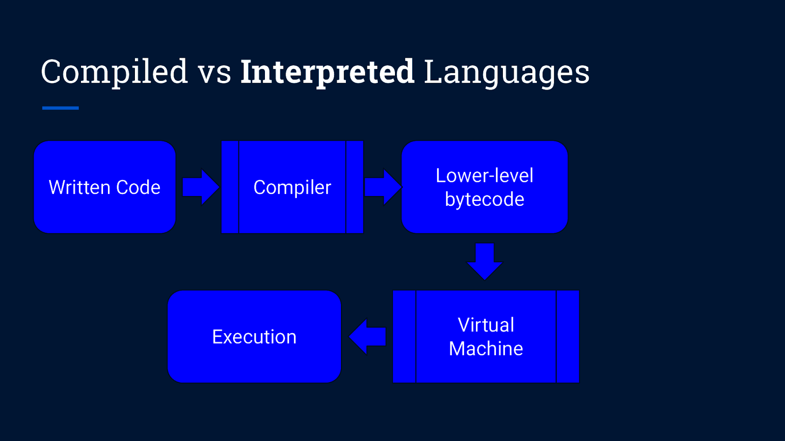
Compiled vs Interpreted Languages Written Code Compiler Execution Lower-level bytecode Virtual Machine

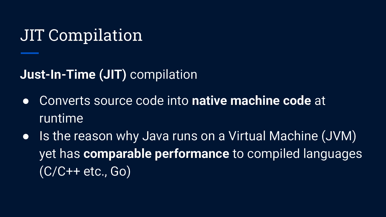
JIT Compilation Just-In-Time (JIT) compilation ● Converts source code into native machine code at runtime ● Is the reason why Java runs on a Virtual Machine (JVM) yet has comparable performance to compiled languages (C/C++ etc., Go)

JIT Compilation in Data Science

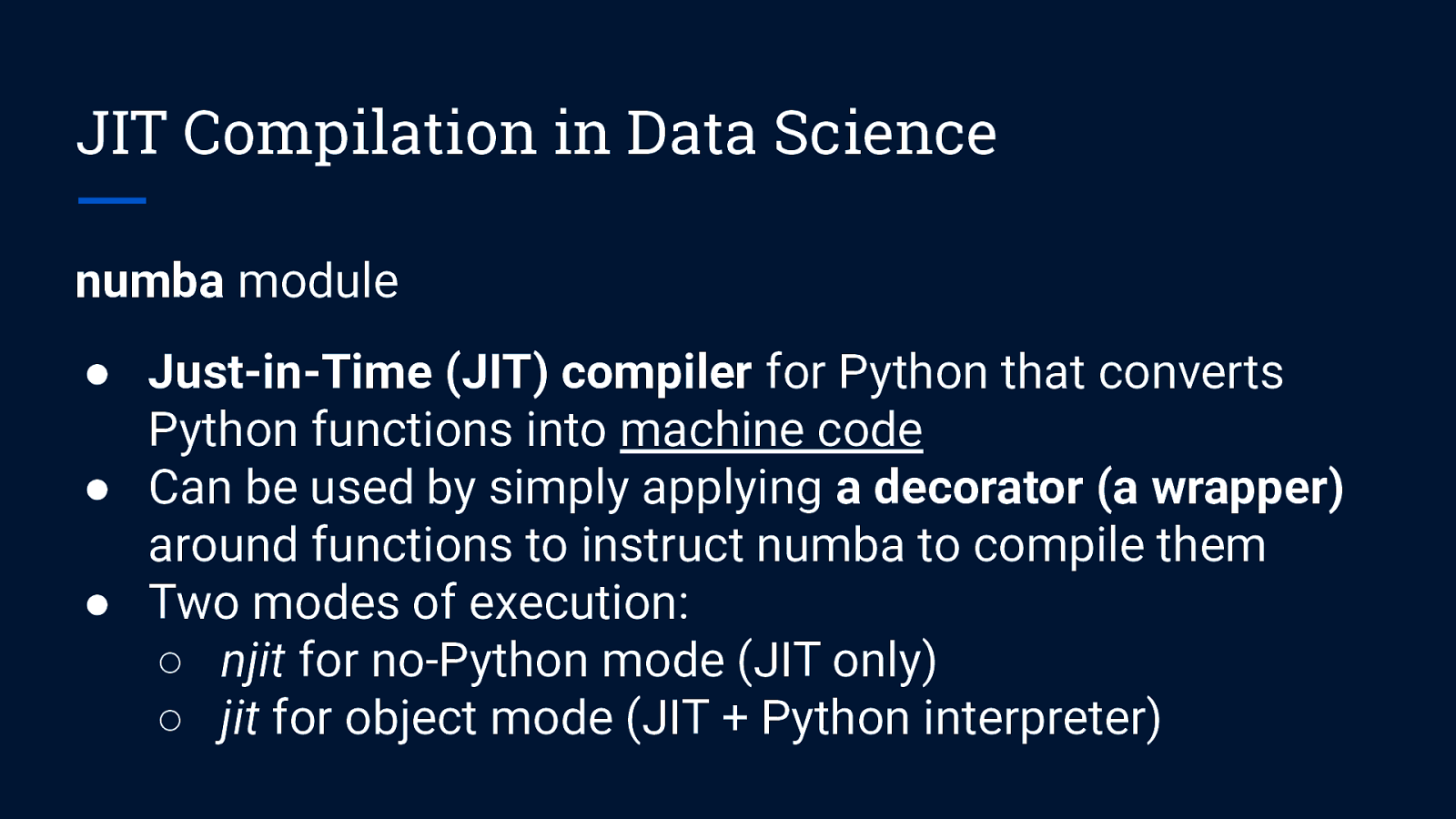
JIT Compilation in Data Science numba module ● Just-in-Time (JIT) compiler for Python that converts Python functions into machine code ● Can be used by simply applying a decorator (a wrapper) around functions to instruct numba to compile them ● Two modes of execution: ○ njit for no-Python mode (JIT only) ○ jit for object mode (JIT + Python interpreter)

Practical Implementation

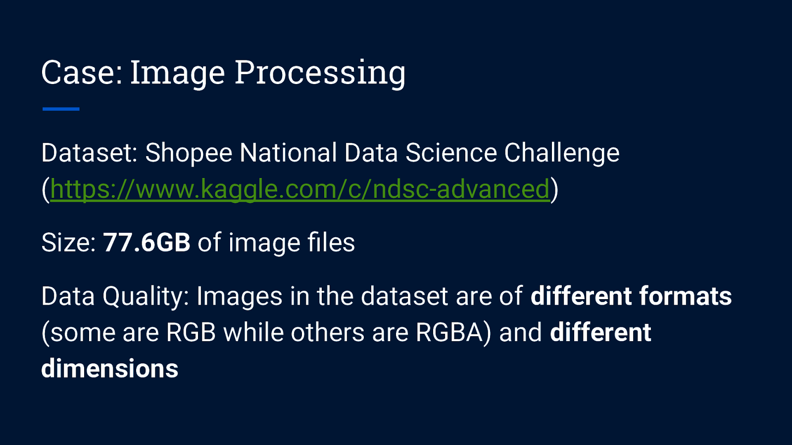
Case: Image Processing Dataset: Shopee National Data Science Challenge (https://www.kaggle.com/c/ndsc-advanced) Size: 77.6GB of image files Data Quality: Images in the dataset are of different formats (some are RGB while others are RGBA) and different dimensions

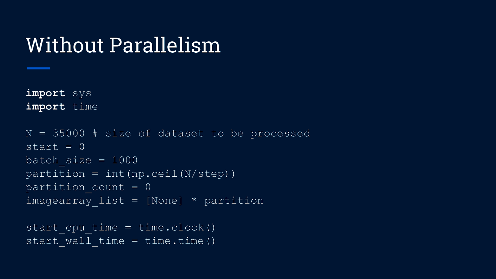
Without Parallelism import sys import time N = 35000 # size of dataset to be processed start = 0 batch_size = 1000 partition = int(np.ceil(N/step)) partition_count = 0 imagearray_list = [None] * partition start_cpu_time = time.clock() start_wall_time = time.time()

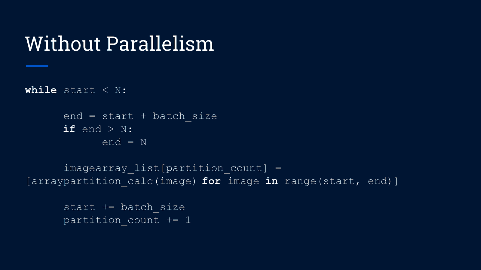
Without Parallelism while start < N: end = start + batch_size if end > N: end = N imagearray_list[partition_count] = [arraypartition_calc(image) for image in range(start, end)] start += batch_size partition_count += 1

Without Parallelism while start < N: end = start + batch_size if end > N: end = N imagearray_list[partition_count] = [arraypartition_calc(image) for image in range(start, end)] start += batch_size partition_count += 1

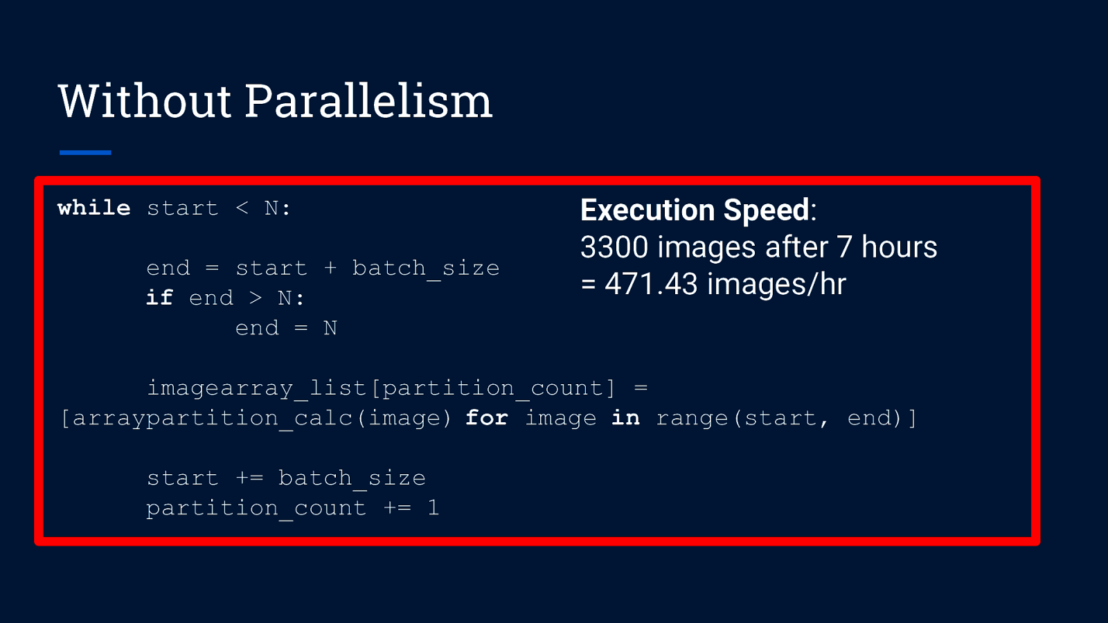
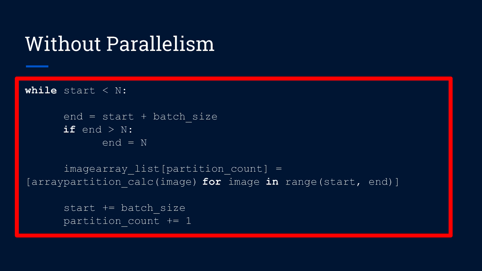
Without Parallelism while start < N: end = start + batch_size if end > N: end = N Execution Speed: 3300 images after 7 hours = 471.43 images/hr imagearray_list[partition_count] = [arraypartition_calc(image) for image in range(start, end)] start += batch_size partition_count += 1

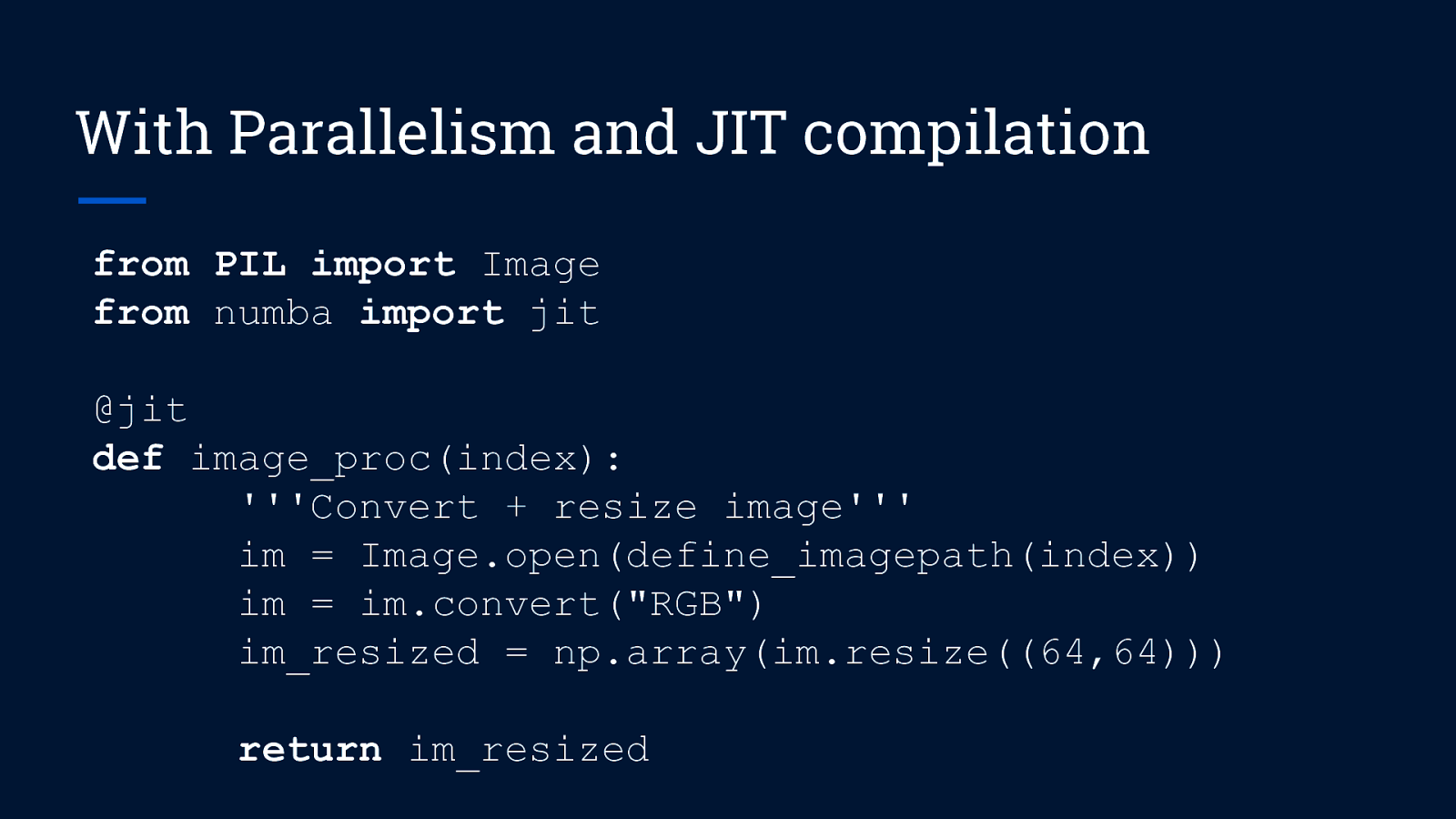
With Parallelism and JIT compilation from PIL import Image from numba import jit @jit def image_proc(index): ”’Convert + resize image”’ im = Image.open(define_imagepath(index)) im = im.convert(“RGB”) im_resized = np.array(im.resize((64,64))) return im_resized

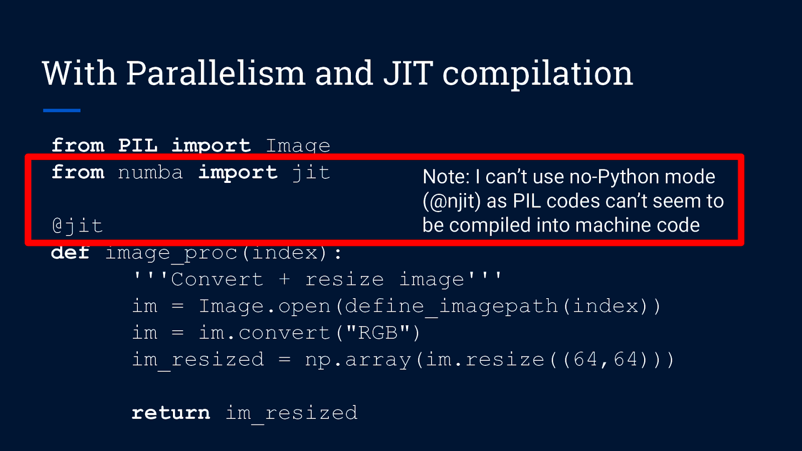
With Parallelism and JIT compilation from PIL import Image from numba import jit Note: I can’t use no-Python mode (@njit) as PIL codes can’t seem to be compiled into machine code @jit def image_proc(index): ”’Convert + resize image”’ im = Image.open(define_imagepath(index)) im = im.convert(“RGB”) im_resized = np.array(im.resize((64,64))) return im_resized

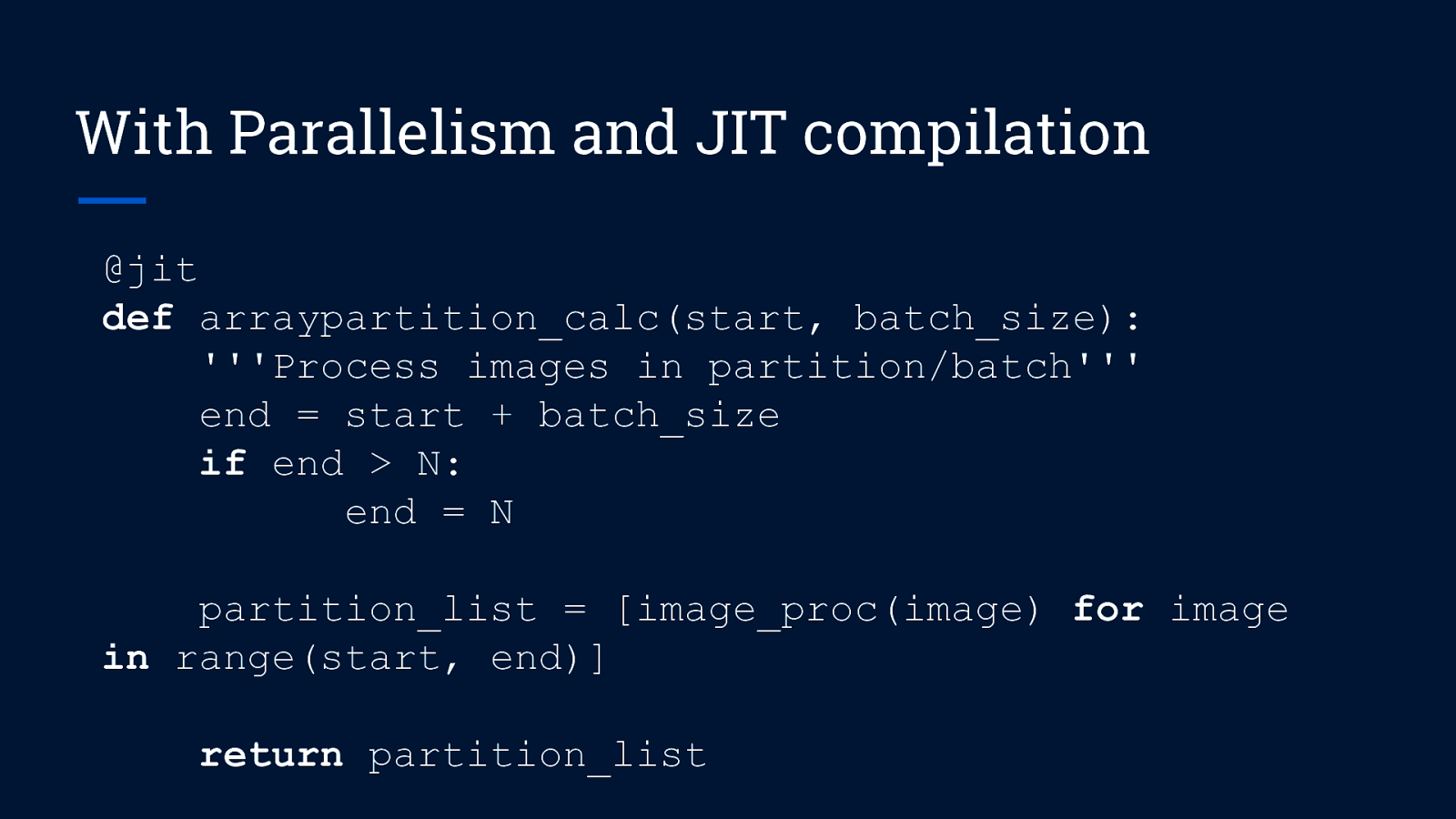
With Parallelism and JIT compilation @jit def arraypartition_calc(start, batch_size): ”’Process images in partition/batch”’ end = start + batch_size if end > N: end = N partition_list = [image_proc(image) for image in range(start, end)] return partition_list

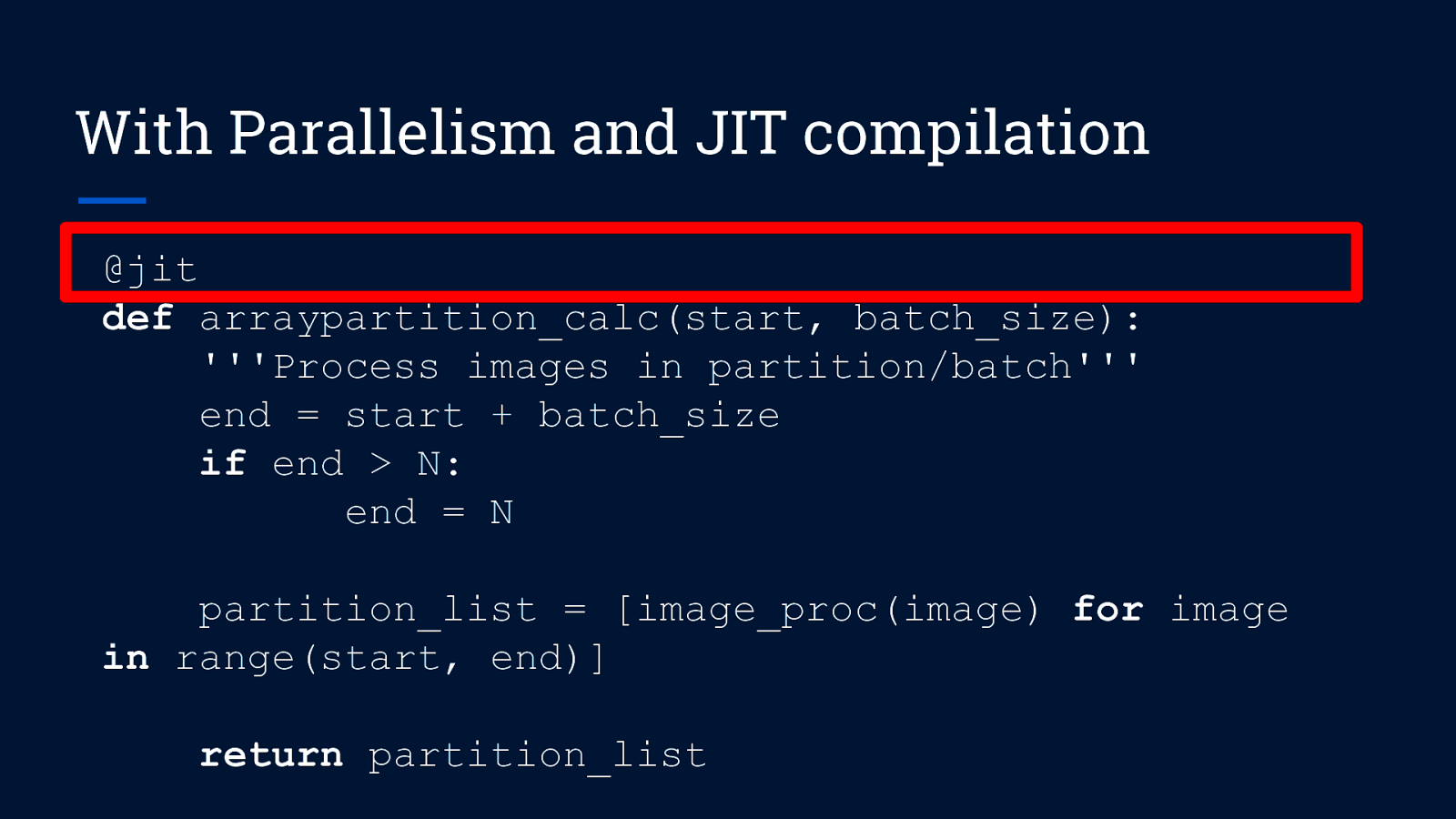
With Parallelism and JIT compilation @jit def arraypartition_calc(start, batch_size): ”’Process images in partition/batch”’ end = start + batch_size if end > N: end = N partition_list = [image_proc(image) for image in range(start, end)] return partition_list

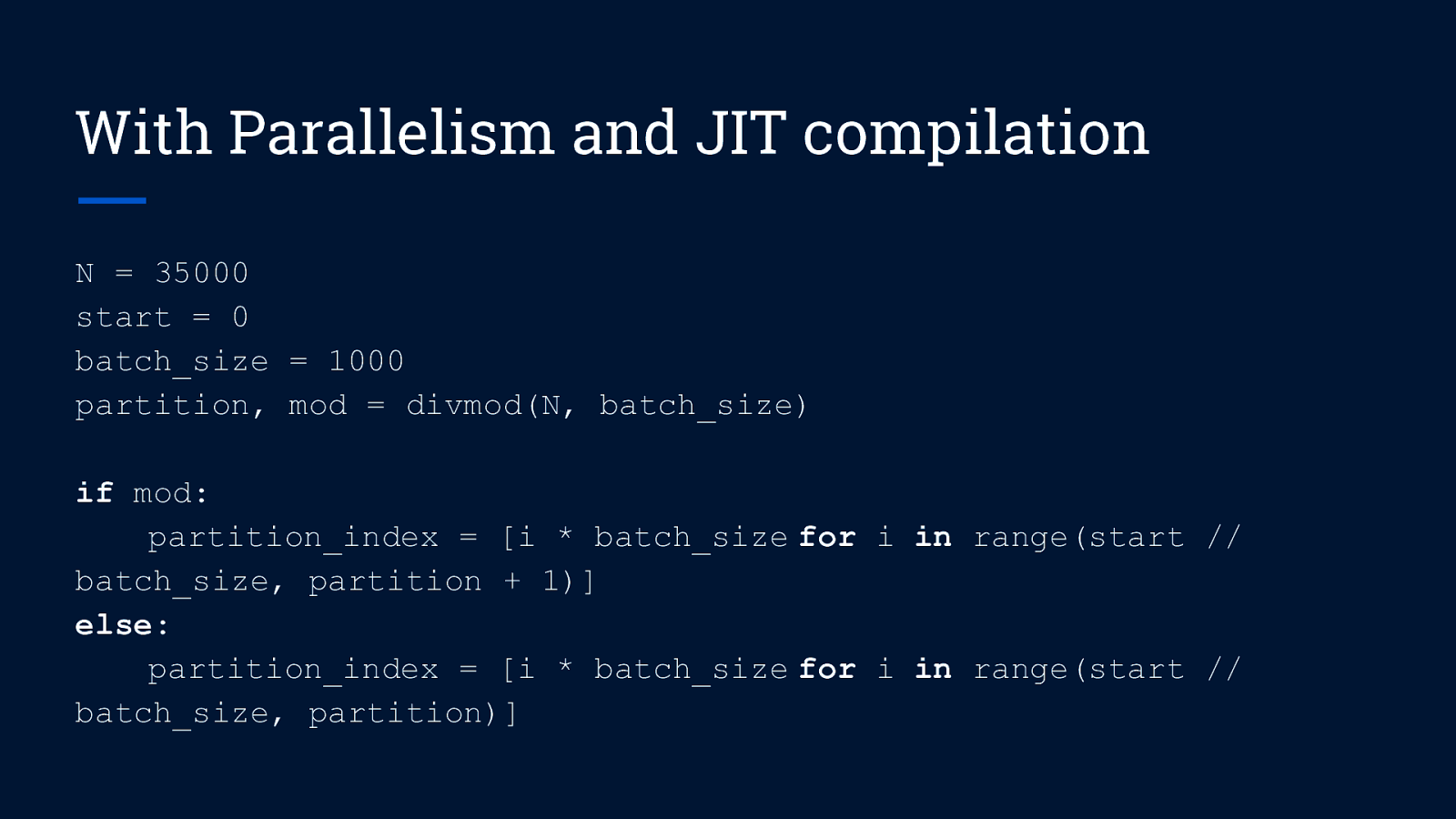
With Parallelism and JIT compilation N = 35000 start = 0 batch_size = 1000 partition, mod = divmod(N, batch_size) if mod: partition_index = [i * batch_size for i in range(start // batch_size, partition + 1)] else: partition_index = [i * batch_size for i in range(start // batch_size, partition)]

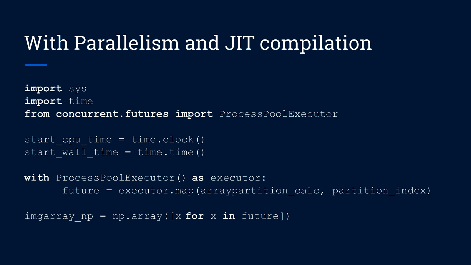
With Parallelism and JIT compilation import sys import time from concurrent.futures import ProcessPoolExecutor start_cpu_time = time.clock() start_wall_time = time.time() with ProcessPoolExecutor() as executor: future = executor.map(arraypartition_calc, partition_index) imgarray_np = np.array([x for x in future])

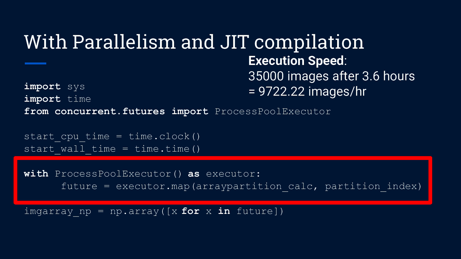
With Parallelism and JIT compilation Execution Speed: 35000 images after 3.6 hours = 9722.22 images/hr import sys import time from concurrent.futures import ProcessPoolExecutor start_cpu_time = time.clock() start_wall_time = time.time() with ProcessPoolExecutor() as executor: future = executor.map(arraypartition_calc, partition_index) imgarray_np = np.array([x for x in future])

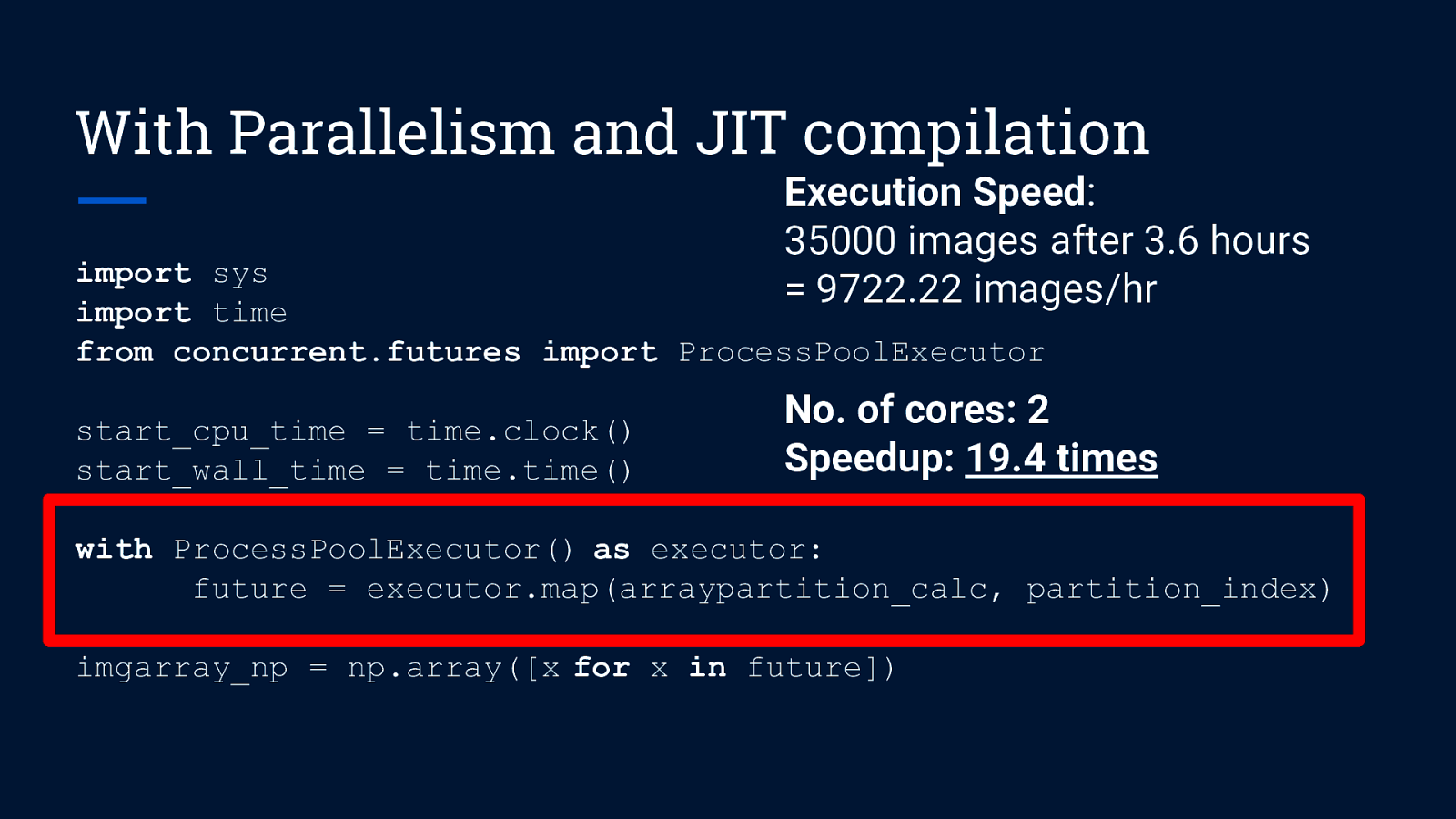
With Parallelism and JIT compilation Execution Speed: 35000 images after 3.6 hours = 9722.22 images/hr import sys import time from concurrent.futures import ProcessPoolExecutor start_cpu_time = time.clock() start_wall_time = time.time() No. of cores: 2 Speedup: 19.4 times with ProcessPoolExecutor() as executor: future = executor.map(arraypartition_calc, partition_index) imgarray_np = np.array([x for x in future])

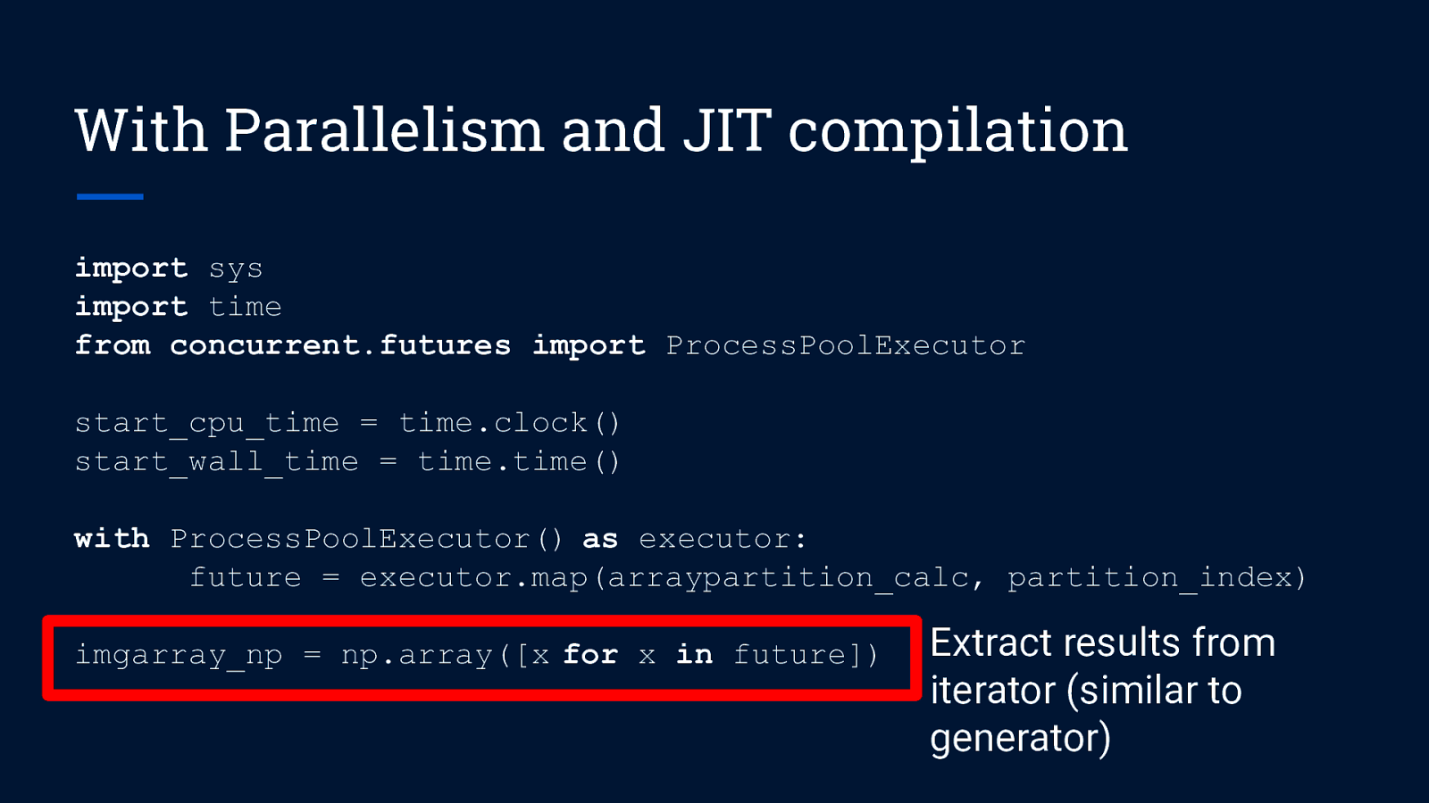
With Parallelism and JIT compilation import sys import time from concurrent.futures import ProcessPoolExecutor start_cpu_time = time.clock() start_wall_time = time.time() with ProcessPoolExecutor() as executor: future = executor.map(arraypartition_calc, partition_index) imgarray_np = np.array([x for x in future]) Extract results from iterator (similar to generator)

Key Takeaways

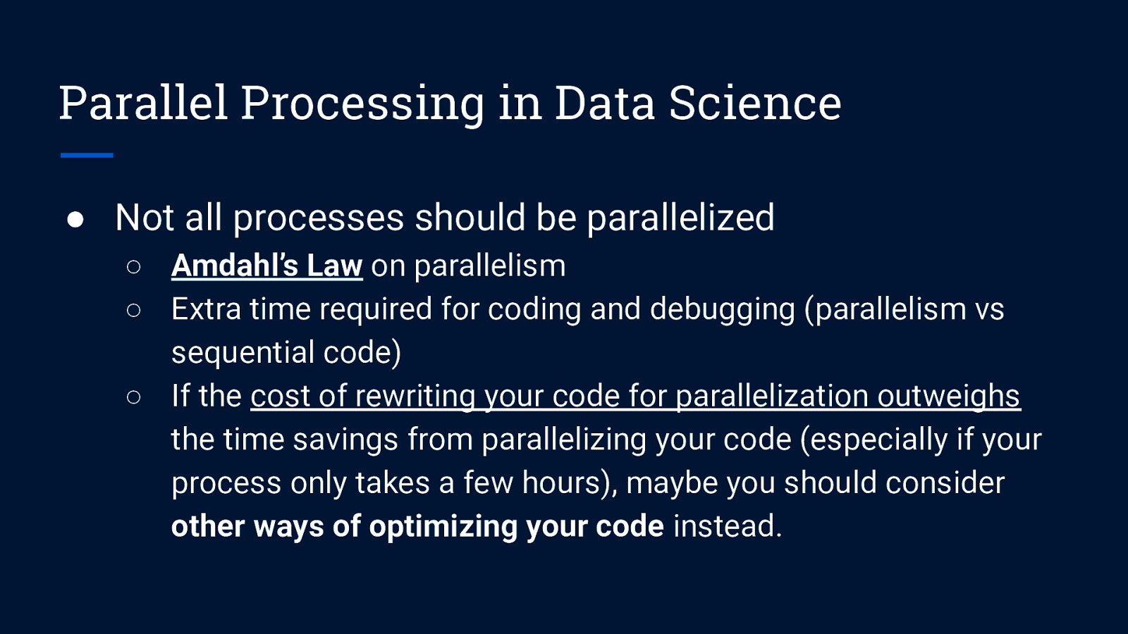
Parallel Processing in Data Science ● Not all processes should be parallelized ○ Amdahl’s Law on parallelism ○ Extra time required for coding and debugging (parallelism vs sequential code) ○ If the cost of rewriting your code for parallelization outweighs the time savings from parallelizing your code (especially if your process only takes a few hours), maybe you should consider other ways of optimizing your code instead.

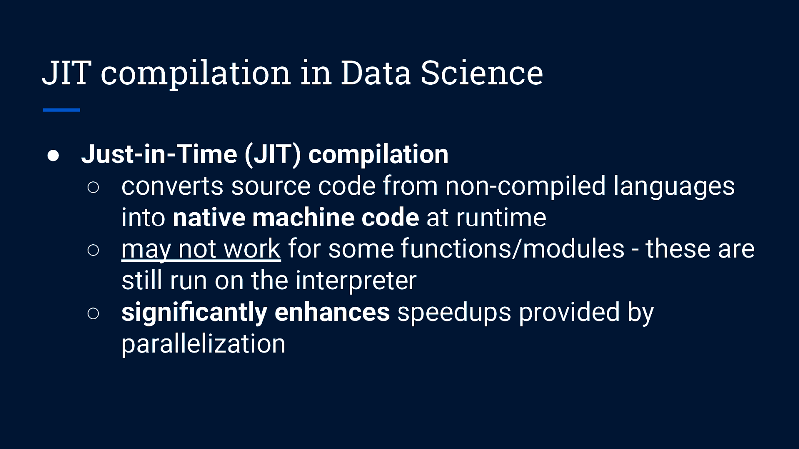
JIT compilation in Data Science ● Just-in-Time (JIT) compilation ○ converts source code from non-compiled languages into native machine code at runtime ○ may not work for some functions/modules - these are still run on the interpreter ○ significantly enhances speedups provided by parallelization

References Official Python documentation on concurrent.futures (https://docs.python.org/3/library/concurrent.futures.html) Built-in Functions - Python 3.7.4 Documentation (https://docs.python.org/3/library/functions.html#map) 5-minute Guide to Numba (http://numba.pydata.org/numba-doc/latest/user/5minguide.html)

Contact Ong Chin Hwee LinkedIn: ongchinhwee Twitter: @ongchinhwee https://ongchinhwee.me