Making an Accessible Excel Workbook
Aaron Farber Accessibility Engineer

A presentation at TPGi Webinar in October 2021 in by Aaron Farber

Aaron Farber Accessibility Engineer

Agenda 1) Introduction 5) Graphs and Charts 2) Structure 6) Accessibility Check/Document Inspector 3) Tables 4) Use of Color 7) Conclusion

Introduction
What’s an accessible document? ▪ An accessible document is one that every person can read, understand, and interact with in a comparable experience. - For example: in a similar amount of time or level of expertise with the program.
Before we get started, understand: ▪ This presentation focuses on making a workbook accessible to people with low-vision or blindness. ▪ In Excel, there are numerous ways to achieve each task. Multiple approaches are valid. ▪ WCAG standards can be mapped to Excel workbooks.
People with low-vision: ▪ May have challenges discerning text or elements, such as within charts/graphs, which have low color contrast. ▪ May magnify the workbook, which necessitates more scrolling and seeing less content at once.
People with blindness: ▪ Primarily navigate using the cursor keys to move one cell in one direction at a time. ▪ Excel’s robust functionalities can be accessed using the popular screen readers, but people may not know the full range of keyboard commands.

Structure
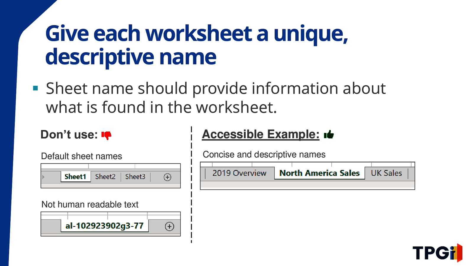
Give each worksheet a unique, descriptive name ▪ Sheet name should provide information about what is found in the worksheet. Don’t use: Accessible Example: Default sheet names Concise and descriptive names screenshot of Excel sheet tabs with names Sheet 1 Sheet 2 Sheet 3 Not human readable text Screenshot of a single sheet tab with unreadable text al-2390230953-24f screenshot of Excel sheet tabs with names 2019 Overview, North America Sales, UK Sales
Do not leave Cell A1 blank ▪ Cell A1 is a critical landmark for structure and navigation. Start content at A1. ▪ When a screen reader user enters a worksheet, the first selected cell is A1. ▪ Cell A1 should be used to orient users to the structure of the workbook or worksheet. ▪ Examples to follow:
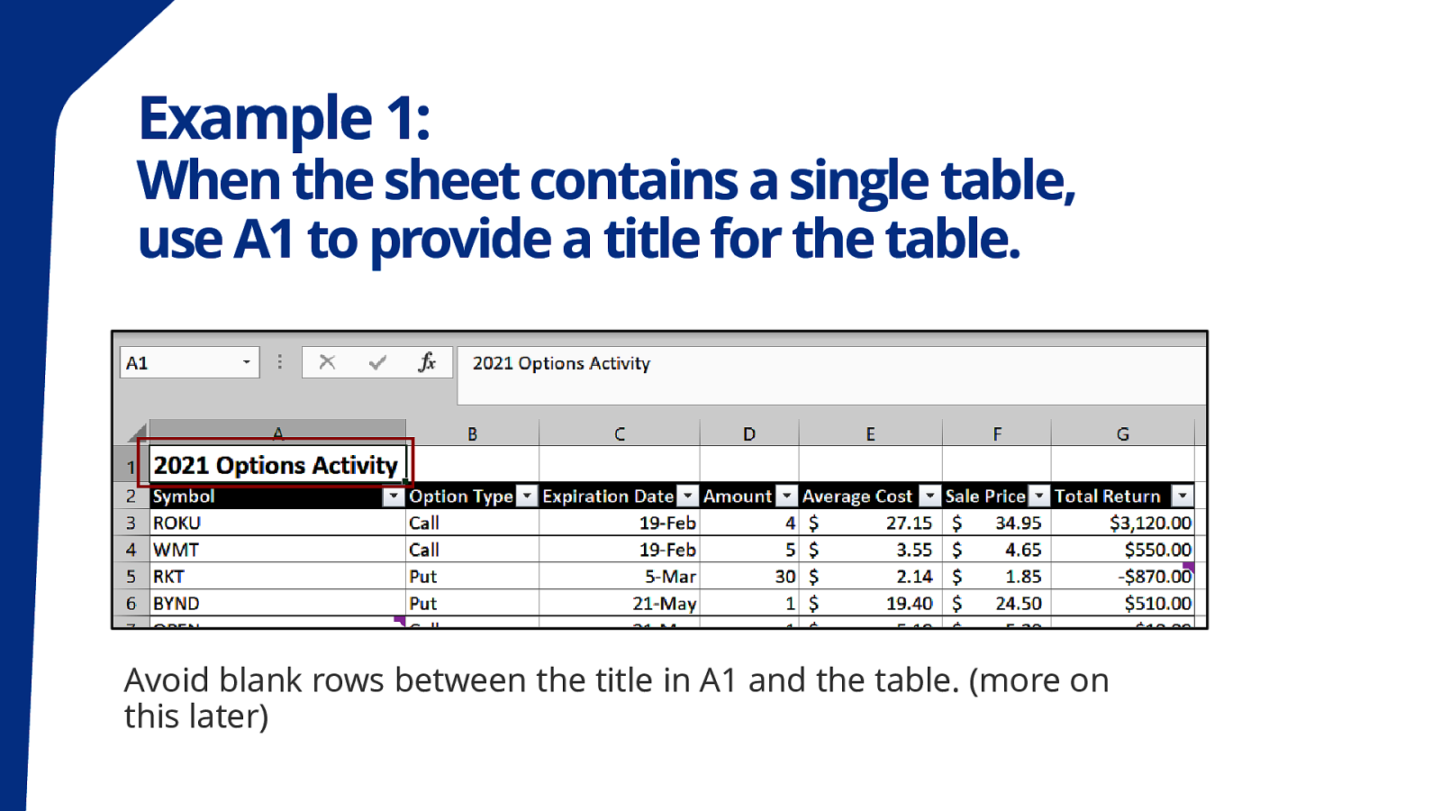
Example 1: When the sheet contains a single table, use A1 to provide a title for the table. Screenshot of Excel shows cell A1 with table title “2021 Options Activity”. The table has seven columns about options information. It also shows several rows of options transactions for example, Roku call option expiring february 2019. Avoid blank rows between the title in A1 and the table. (more on this later)
Example 2: When the workbook/worksheet has a more complex structure, provide a text summary. ▪ To aid screen reader users, the text summary should describe the workbook or worksheet’s structure. ▪ When a sheets has multiple tables or sections, the summary should state the cell where each element starts. ▪ The summary should note if the worksheet contains charts/graphs, images, anything interactive, or irregular.
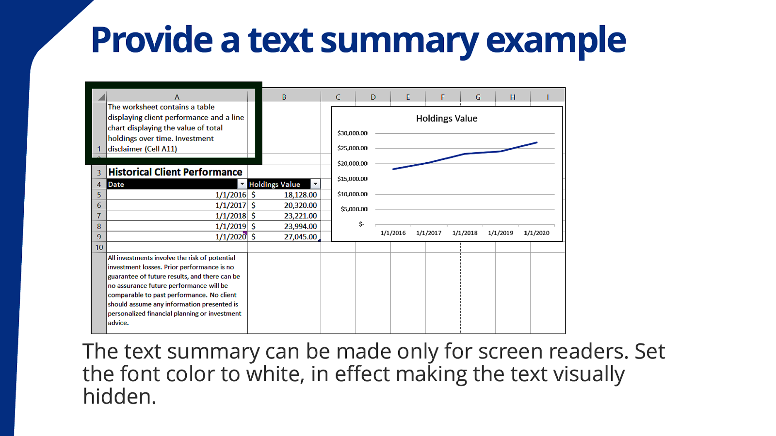
Provide a text summary example Screenshot of Excel worksheet. Cell A1 includes a text summary “The worksheet contains a table displaying client performance and a line chart displaying the value of total holdings over time. Investment disclaimer (Cell A11)”. It is a complex workbook with multiple elements. The text summary can be made only for screen readers. Set the font color to white, in effect making the text visually hidden.
Simplify your workbook ▪ When a worksheet has multiple sections or tables, separate each element by a single row. Avoid multiple blanks rows/columns. ▪ When multiple rows separate elements, screen reader users may reach the end of a table/section and not know there is more content further down the worksheet.
Hide unused rows, columns outside the working area ▪ This prevents users from wandering into parts of the worksheet that are not being used. ▪ It reduces the workbook’s file size, making the file more performative. ▪ Do not hide rows/columns within the working area. ▪ Do not merge cells. This disrupts screen reader users’ navigation and understanding of where they are located within the spreadsheet.
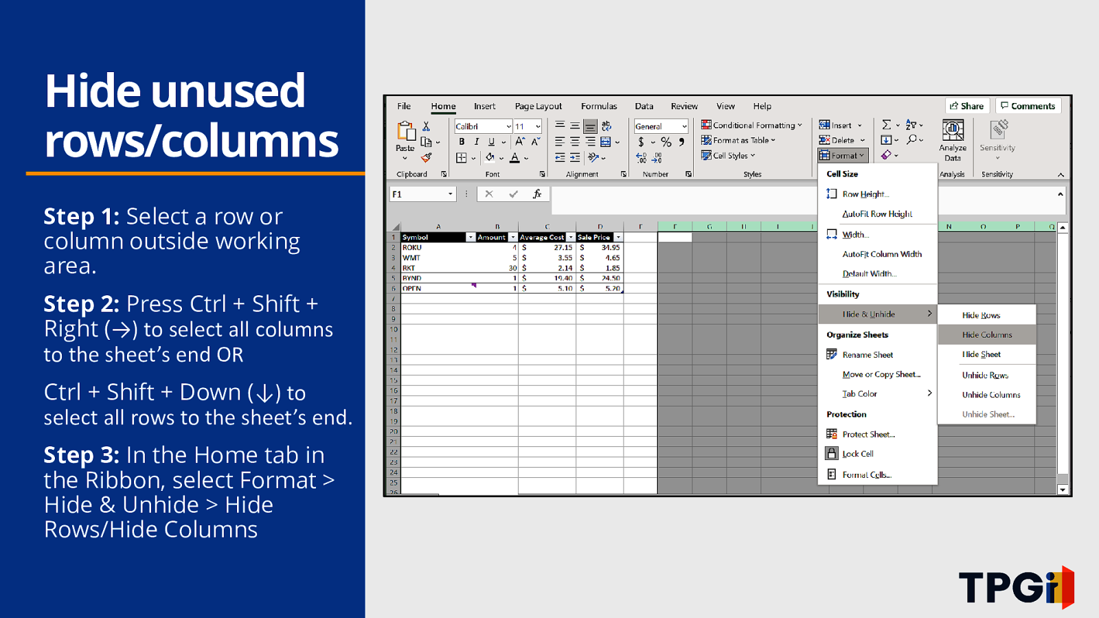
Hide unused rows/columns Step 1: Select a row or column outside working area. Step 2: Press Ctrl + Shift + Right (→) to select all columns to the sheet’s end OR Ctrl + Shift + Down (↓) to select all rows to the sheet’s end. Step 3: In the Home tab in the Ribbon, select Format > Hide & Unhide > Hide Rows/Hide Columns screenshot shows a table which ends at column D. Column F to the right end of the worksheet is selected. in the Excel Ribbon, Home tab, the Format dropdown is extended. Hide and Unhid is an option.

Tables
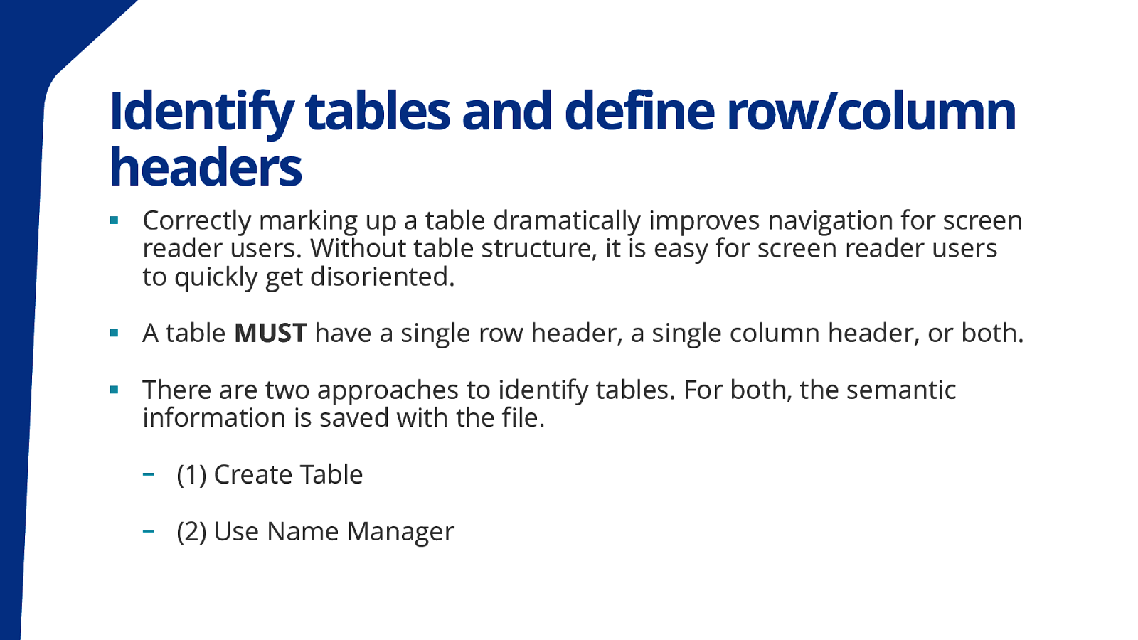
Identify tables and define row/column headers ▪ Correctly marking up a table dramatically improves navigation for screen reader users. Without table structure, it is easy for screen reader users to quickly get disoriented. ▪ A table MUST have a single row header, a single column header, or both. ▪ There are two approaches to identify tables. For both, the semantic information is saved with the file. - (1) Create Table - (2) Use Name Manager
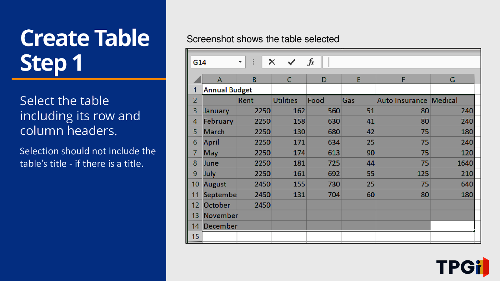
Create Table Step 1 Select the table including its row and column headers. Selection should not include the table’s title - if there is a title. Screenshot shows the table selected Screenshot of Excel worksheet. Cell A1 has table title Annual Budget. The table starting at B1 is selected from the column header titles to the last row.
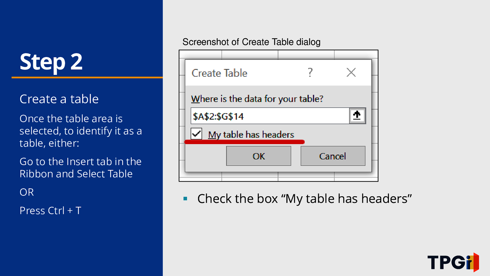
Step 2 Screenshot of Create Table dialog Create a table Once the table area is selected, to identify it as a table, either: Go to the Insert tab in the Ribbon and Select Table OR Press Ctrl + T ▪ Check the box “My table has headers”
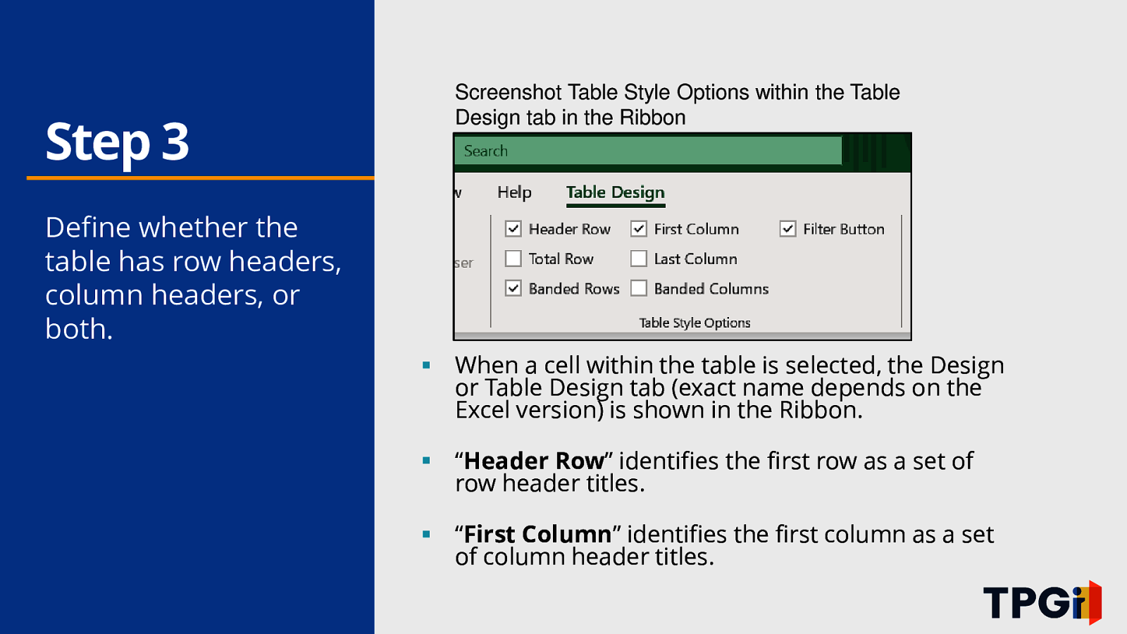
Step 3 Define whether the table has row headers, column headers, or both. Screenshot Table Style Options within the Table Design tab in the Ribbon Table Design tab shows header row and first column checkboxes checked. ▪ When a cell within the table is selected, the Design or Table Design tab (exact name depends on the Excel version) is shown in the Ribbon. ▪ “Header Row” identifies the first row as a set of row header titles. ▪ “First Column” identifies the first column as a set of column header titles.
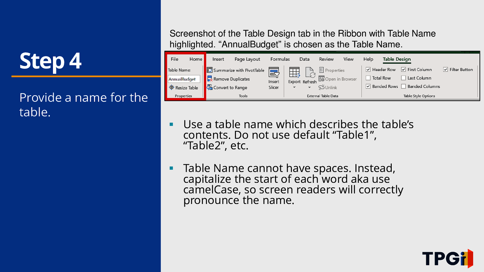
Step 4 Provide a name for the table. Screenshot of the Table Design tab in the Ribbon with Table Name highlighted. “AnnualBudget” is chosen as the Table Name. ▪ Use a table name which describes the table’s contents. Do not use default “Table1”, “Table2”, etc. ▪ Table Name cannot have spaces. Instead, capitalize the start of each word aka use camelCase, so screen readers will correctly pronounce the name.
Step 5 Turn on a screen reader and test! ▪ When a table is identified and its row/column header titles are defined: - Screen readers (JAWS 2021 and Windows’ built-in screen reader Narrator) announce each cell’s value AND its associated row/column headers. - Upon entering the table, screen readers announce the name of the table and the number of rows, columns.
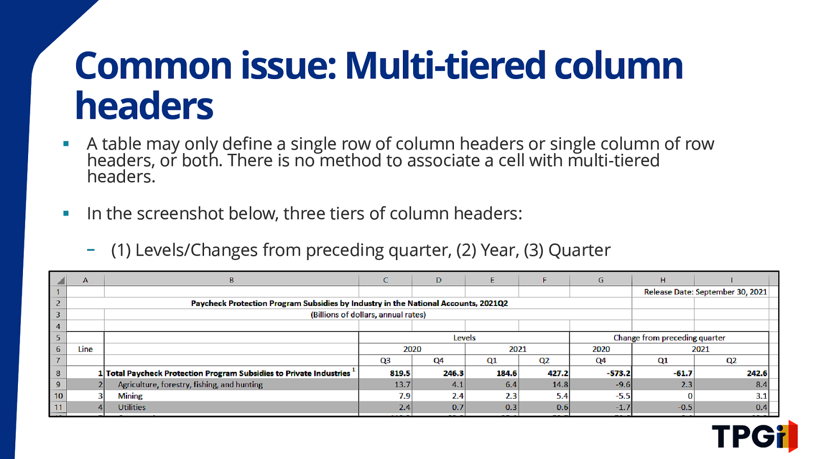
Common issue: Multi-tiered column headers ▪ A table may only define a single row of column headers or single column of row headers, or both. There is no method to associate a cell with multi-tiered headers. ▪ In the screenshot below, three tiers of column headers: - (1) Levels/Changes from preceding quarter, (2) Year, (3) Quarter Paycheck Protection Program Subsidies by Industry in the National Accounts, 2021 table. The table has three tiers of column headers. First tier “levels” and “Change from preceding quarter”. Second tier “2020”, “2021”, “2020”, and “2021”. Third tier is “Q3”, “Q4”, “Q1”, “Q2”, “Q4”, “Q1”, and “Q2”. The row title headers is industries. It’s a complex table.

Solutions to multi-tiered headers ▪ Option 1: - Break up the complex table into smaller tables ▪ Option 2: - Apply screen reader-only (visually hidden) text within each header title to provide an extended and more descriptive title.
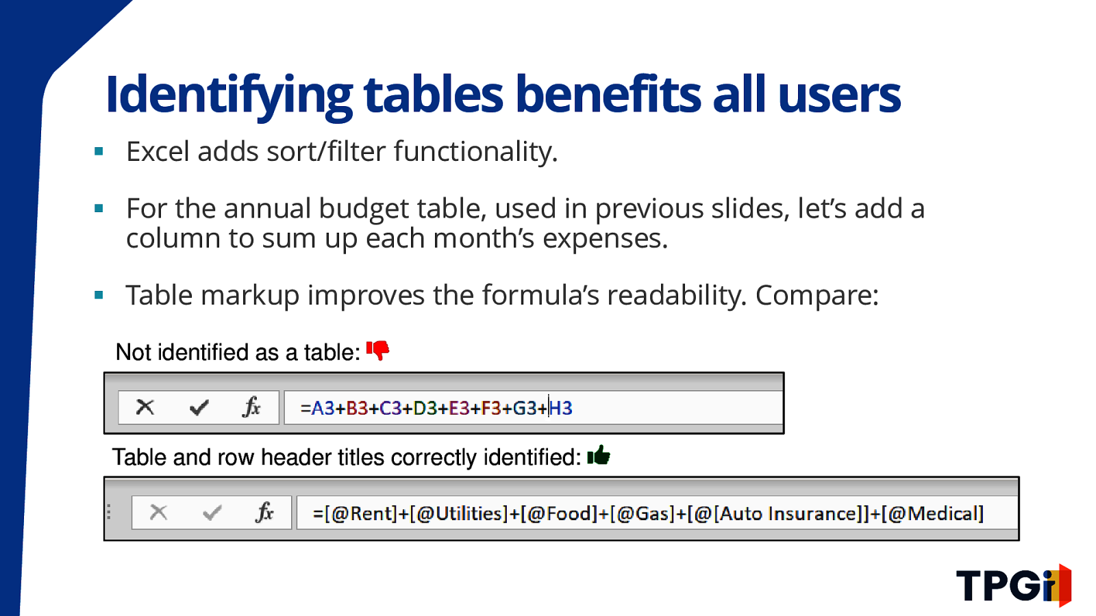
Identifying tables benefits all users ▪ Excel adds sort/filter functionality. ▪ For the annual budget table, used in previous slides, let’s add a column to sum up each month’s expenses. ▪ Table markup improves the formula’s readability. Compare: Not identified as a table: Formula reads A3 + B3 + C3 + D3 + E3 + F3 + G3 + H3 Table and row header titles correctly identified: Formula reads @Rent + @Utilities + @Food + @Gas + @Auto Insurance + @Medical
Use Name Manager • Excel has a built-in syntax to give names to a range of cells and build row/column titles into the workbook. • Every region within the spreadsheet should have a name. Names must be unique. • Create Table is more straightforward but Name Manager can be used more broadly.
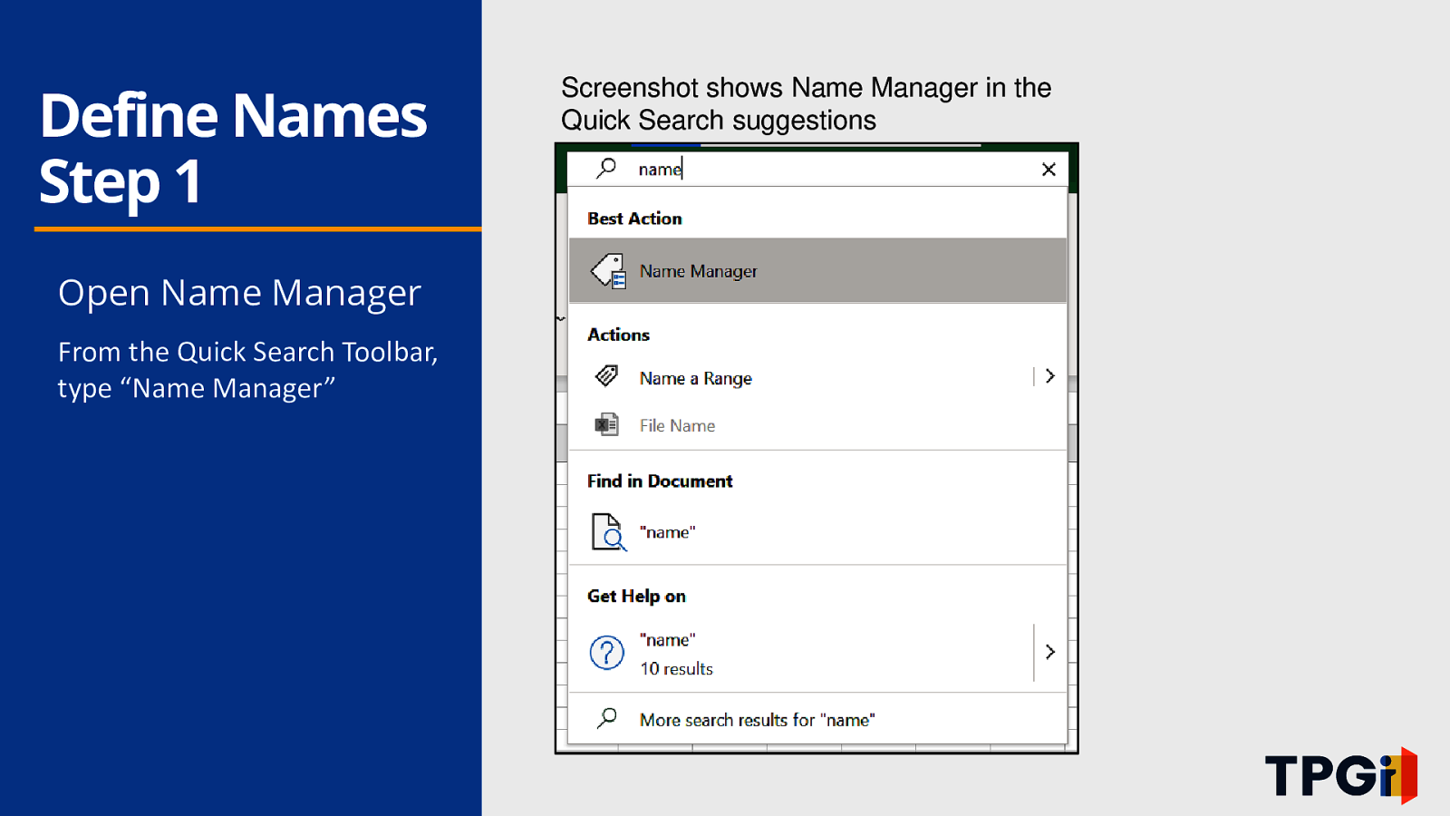
Define Names Step 1 Open Name Manager From the Quick Search Toolbar, type “Name Manager” Screenshot shows Name Manager in the Quick Search suggestions
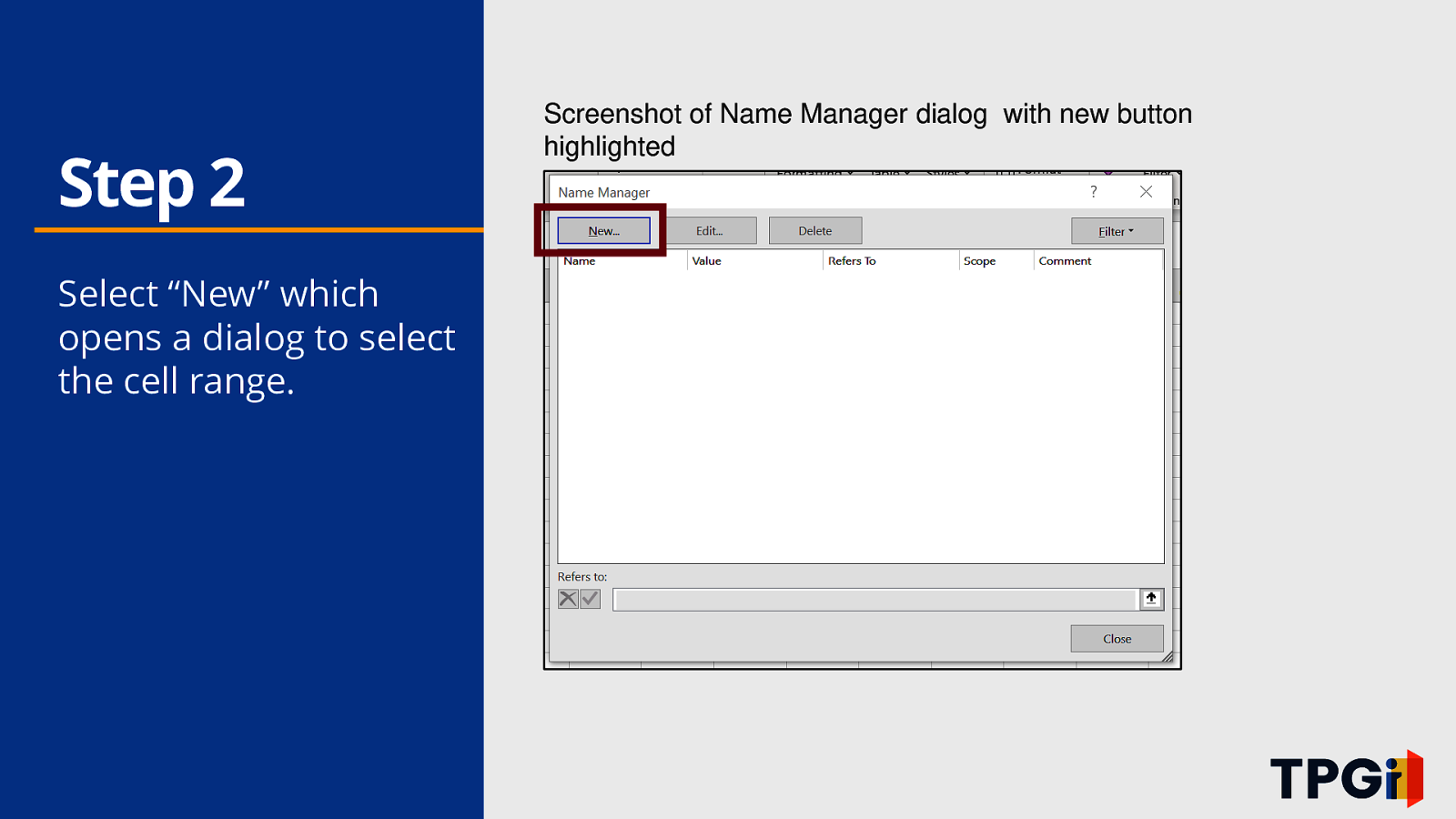
Step 2 Select “New” which opens a dialog to select the cell range. Screenshot of Name Manager dialog with new button highlighted
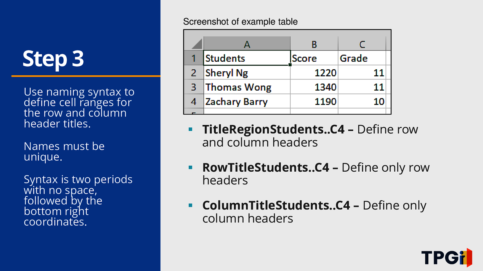
Screenshot of example table Step 3 Use naming syntax to define cell ranges for the row and column header titles. Names must be unique. Syntax is two periods with no space, followed by the bottom right coordinates. ▪ TitleRegionStudents..C4 – Define row and column headers ▪ RowTitleStudents..C4 – Define only row headers ▪ ColumnTitleStudents..C4 – Define only column headers

Use of Color
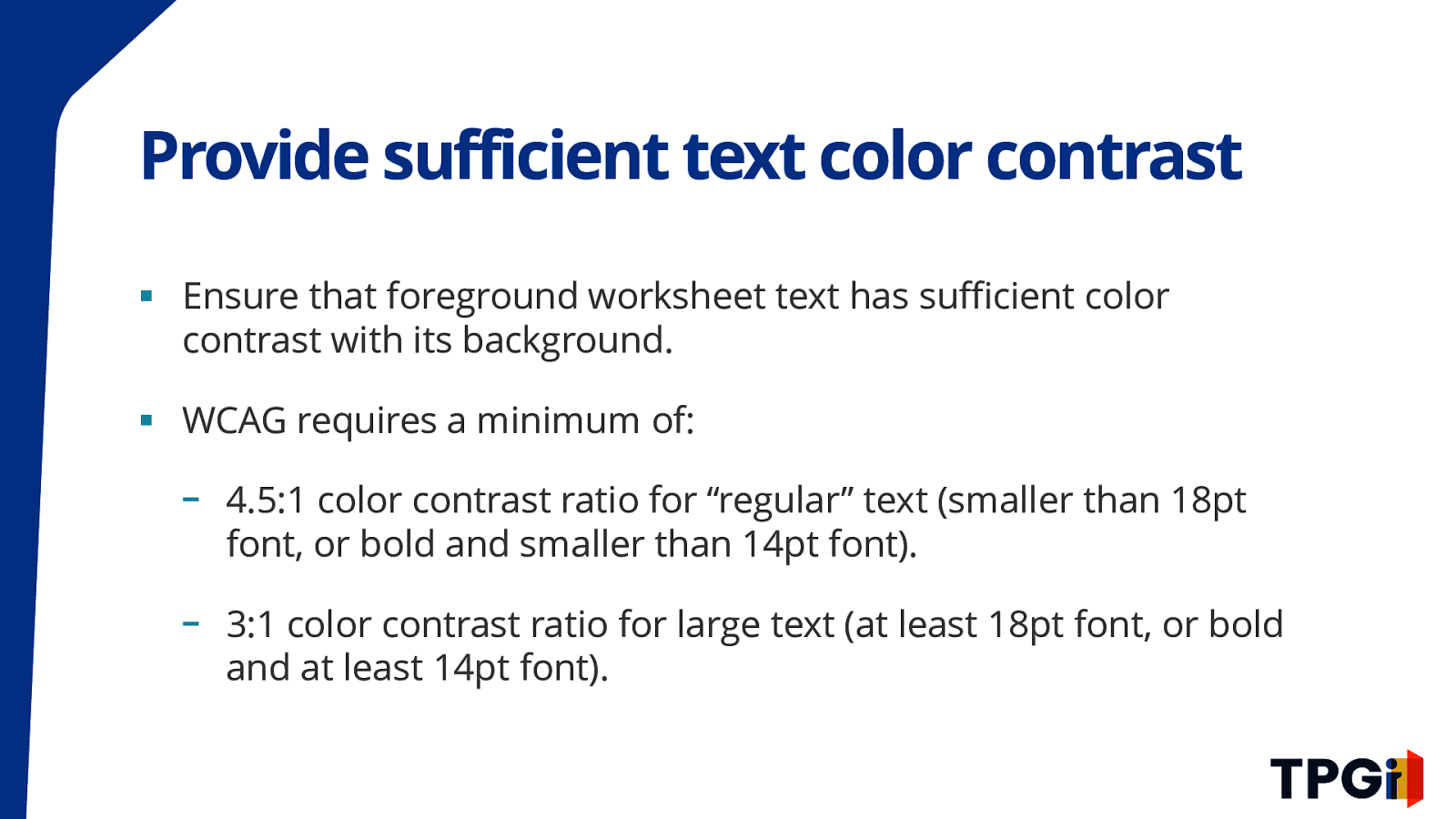
Provide sufficient text color contrast ▪ Ensure that foreground worksheet text has sufficient color contrast with its background. ▪ WCAG requires a minimum of: - 4.5:1 color contrast ratio for “regular” text (smaller than 18pt font, or bold and smaller than 14pt font). - 3:1 color contrast ratio for large text (at least 18pt font, or bold and at least 14pt font).
Do not use color alone to convey meaning ▪ Screen readers do not announce that a cell has a different background color or foreground text color. ▪ When a table uses color and conditional formatting, use the text summary in A1 to state which cells have additional meaning. ▪ Alternatively, place screen reader-only text within the cell to indicate the meaning conveyed by the color.
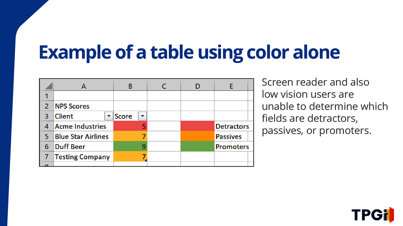
Example of a table using color alone screenshot shows NPS Scores table with two column headers. First column Client Second column score. There are four rows of made up companies. The scores are 5, 7, 9, and 7. 5 cell is colored red. 7 cell is colored yellow. 9 is colored green. There is an adjacent visual legend. Screen reader and also low vision users are unable to determine which fields are detractors, passives, or promoters.
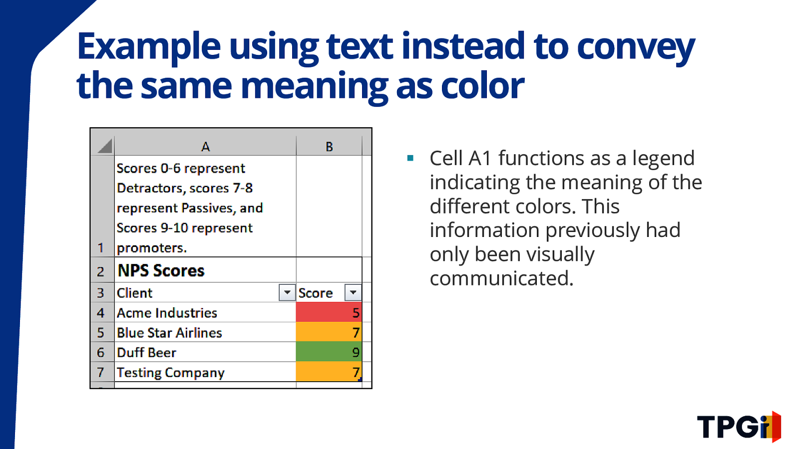
Example using text instead to convey the same meaning as color Text summary in Cell A1 reads “Scores 0-6 represents Detractors”, There is then the NPS scores table. ▪ Cell A1 functions as a legend indicating the meaning of the different colors. This information previously had only been visually communicated.

Graphs / Charts
Excel has a cell layer and a floating layer ▪ When a worksheet has charts, graphs, or images, these objects are in the floating layer. They are not a part of an individual cell. ▪ Screen reader users may not be aware of the content. Screen readers are not notified that there is content in the floating layer. A screen reader user must actively move to the floating layer to find the content. ▪ Navigating to the floating layer is cumbersome.
Provide alternative text for the chart/graph ▪ Do not display charts/graphs alone. Always provide the object’s meaning in an equivalent format i.e. accessible data table. ▪ Alternative text can be applied to floating objects but screen readers may not encounter the alternative text. ▪ In addition, provide alternative text in the cell layer. Cell A1 is a logical outlet.
Use of color in charts / graphs ▪ Charts and graphs present challenges to people that are low-vision or have some level of color blindness. Charts often rely on people perceiving color. ▪ Provide data labels that are always visually present. ▪ Use patterns, e.g. dotted lines or striped bars, to visually identify different chart elements. Color is not required to understand this meaning.

Accessibility Checker / Document Inspector
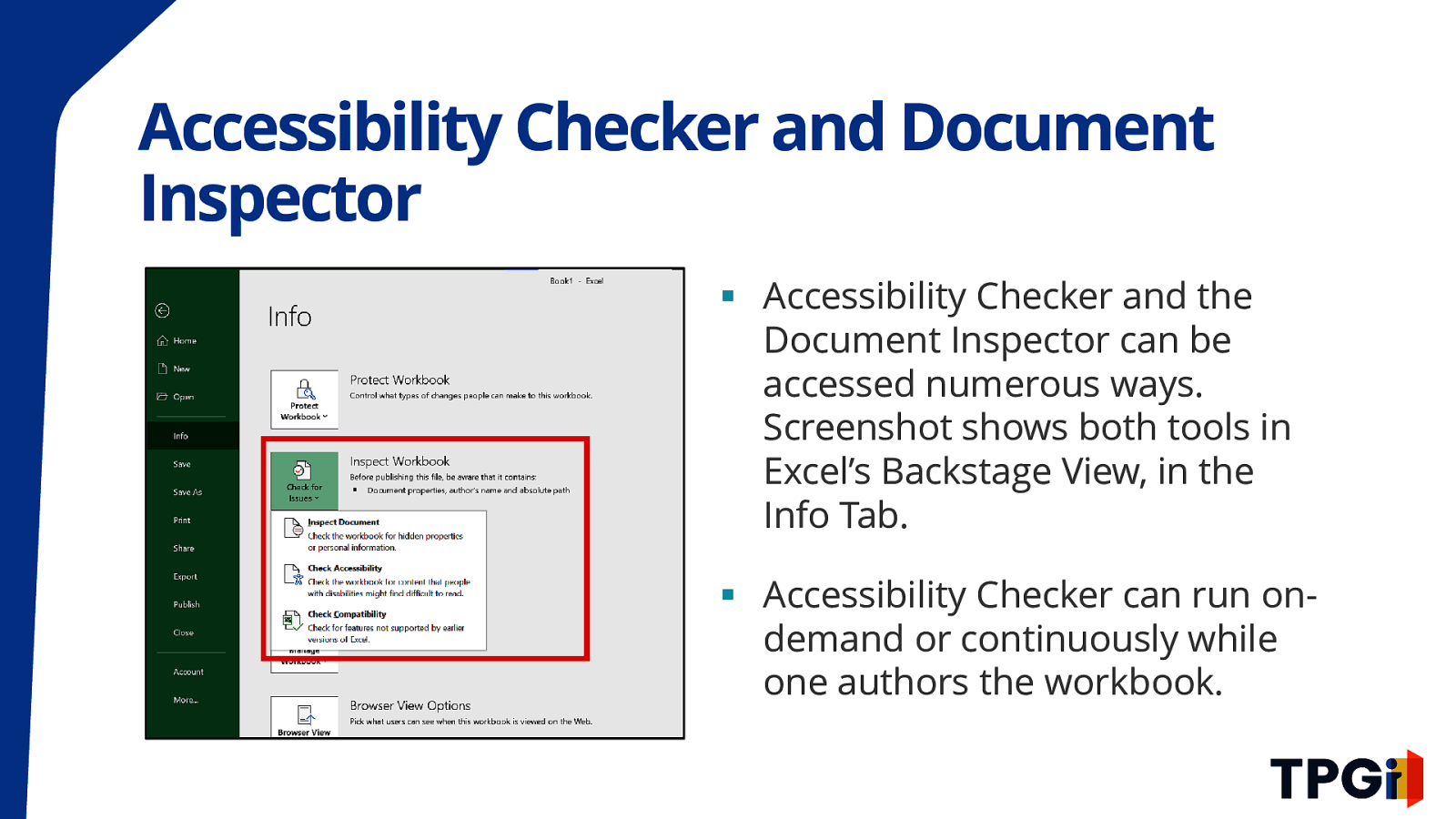
Accessibility Checker and Document Inspector ▪ Accessibility Checker and the Document Inspector can be accessed numerous ways. Screenshot shows both tools in Excel’s Backstage View, in the Info Tab. ▪ Accessibility Checker can run ondemand or continuously while one authors the workbook.
Accessibility Checker is helpful but understand its limitations. - Automated testing is good at detecting occurrences of simple issues but has significant gaps in testing coverage; manual testing is always required. - Examples to follow:
More on Accessibility Checker - The checker flags default sheet names but does not cite nondescriptive or non-readable sheet names as errors or warnings. - Flags lack of alternative text, but cannot evaluate the quality of the alternative text. - Flags hard-to-read cell text with low color contrast but does not test charts/graphs, images - Lack of content in cell A1 is not identified as an error or a warning. - Tables and row/column headers not being defined is not identified as an error or warning.
Document Settings ▪ In Document Properties, reachable from Excel’s Backstage view, provide a title, subject, author, and language. Authors may also add keywords/tags if they so choose. ▪ Document Inspector helps authors prepare a workbook for distribution. Inspector makes authors aware of any comments, revision data, notes and can strip them out this information which is not intended for end users.

Conclusion
Does WCAG apply? ▪ WCAG does not directly apply to Excel. ▪ However, if your website/application hosts Excel workbooks, then WCAG arguably applies. Ultimately, site authors are responsible for all content in their website or application. ▪ Even if the spreadsheet is not publicly available, internal employees require accessible documents. The inability to work with an internal document represents an accessibility issue.
Should you use Excel? ▪ HTML is most accessible. ▪ For websites, allowing users to download workbook to access a simple table, HTML is a more lightweight way of providing the tabular information. ▪ Excel fundamentally makes an assumption about the programs, tools available to the user. Not every person has Excel. ▪ Excel does not work as well with assistive technologies when used on Mac.
Excel has many exciting new features ▪ Data From Picture - Does not produce accessible output by default ▪ Analyze Data - Requires that tables are simple and correctly structured. Has trouble with more complex tables.
Document Remediation and Trainings Available ▪ Word Accessibility ▪ PowerPoint Accessibility ▪ Excel Accessibility ▪ InDesign Accessibility ▪ Accessible Source Document Fundamentals ▪ PDF Accessibility ▪ Advanced PDF Accessibility

Thanks for all the help! - Freedom Scientific @FreedomSci - Microsoft Accessibility @MSFTEnable - Zhi Huang, Access Ingenuity

Questions?